[1] 0 [1] 0 0 1 1 0 0 1 0 1 1 [1] 0 0 0 1 0 0 1 1 1 0 [1] 0 1 1 0 0 0 1 1 1 0Digging a bit deeper
2024-09-11
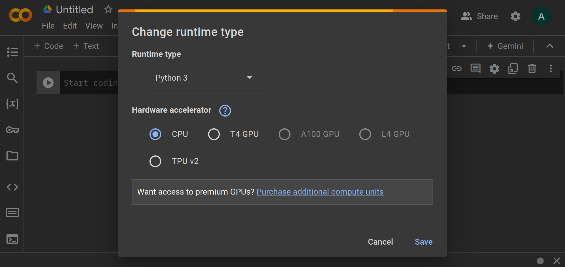
Default is Python 3. Change to R. You’re done with setup.
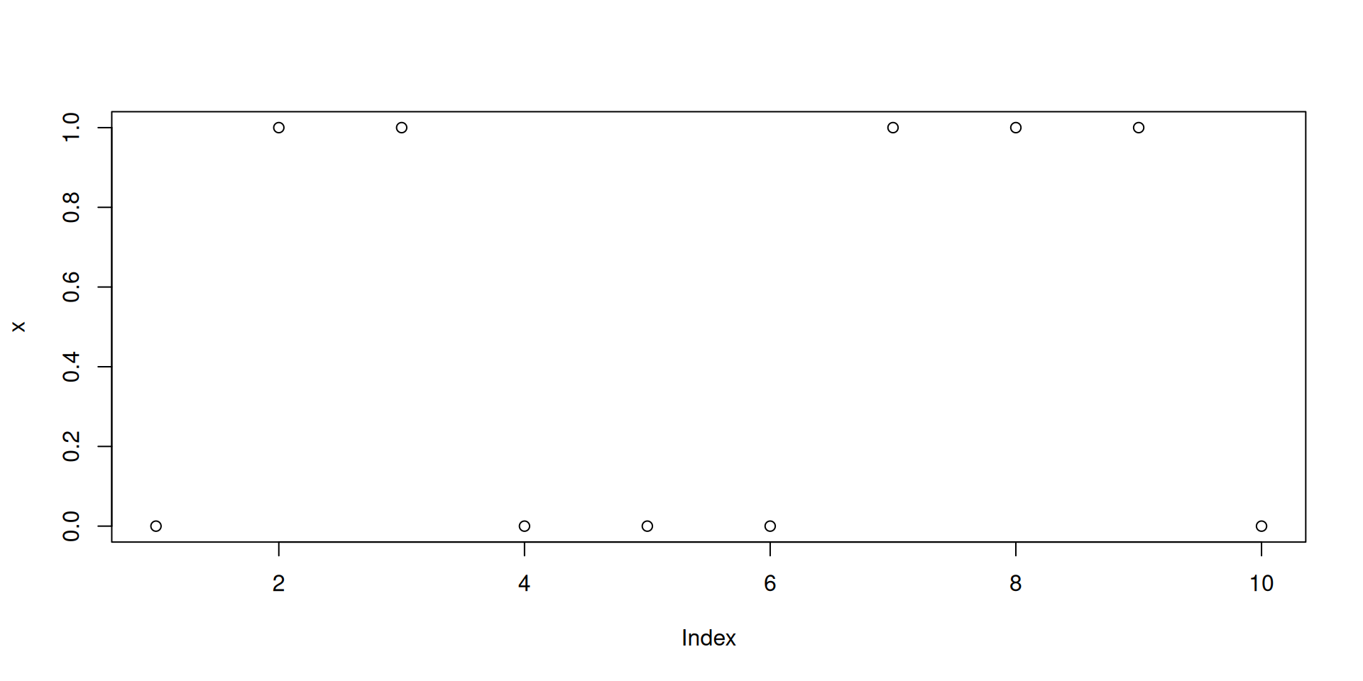
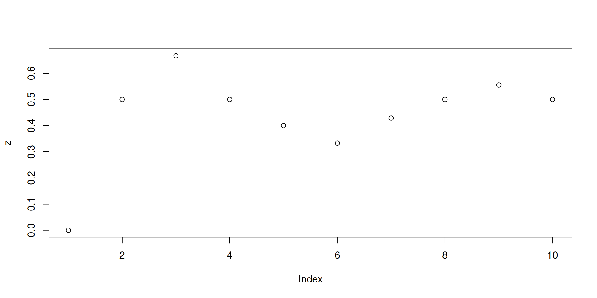
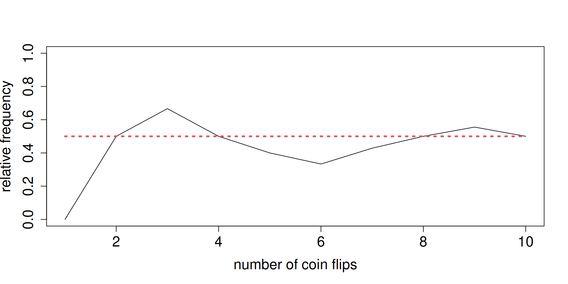
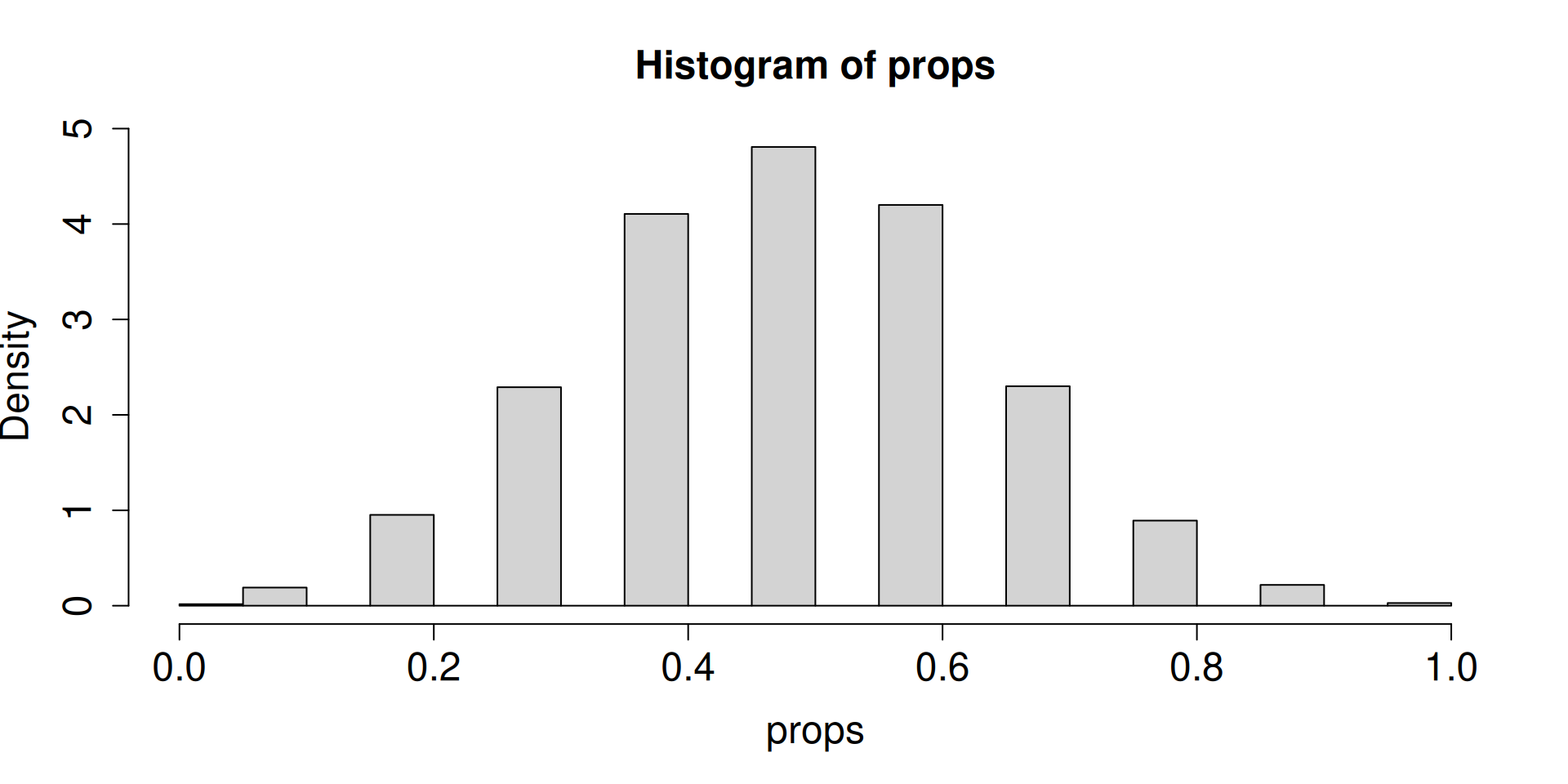
x <- rbinom(10, 1, 0.5).z <- cumsum(x)/(1:length(x)) is really calculating a sequence of relative frequencies.Pretend that “the dog chooses the correct cup” is like “getting Heads in a coin toss”.
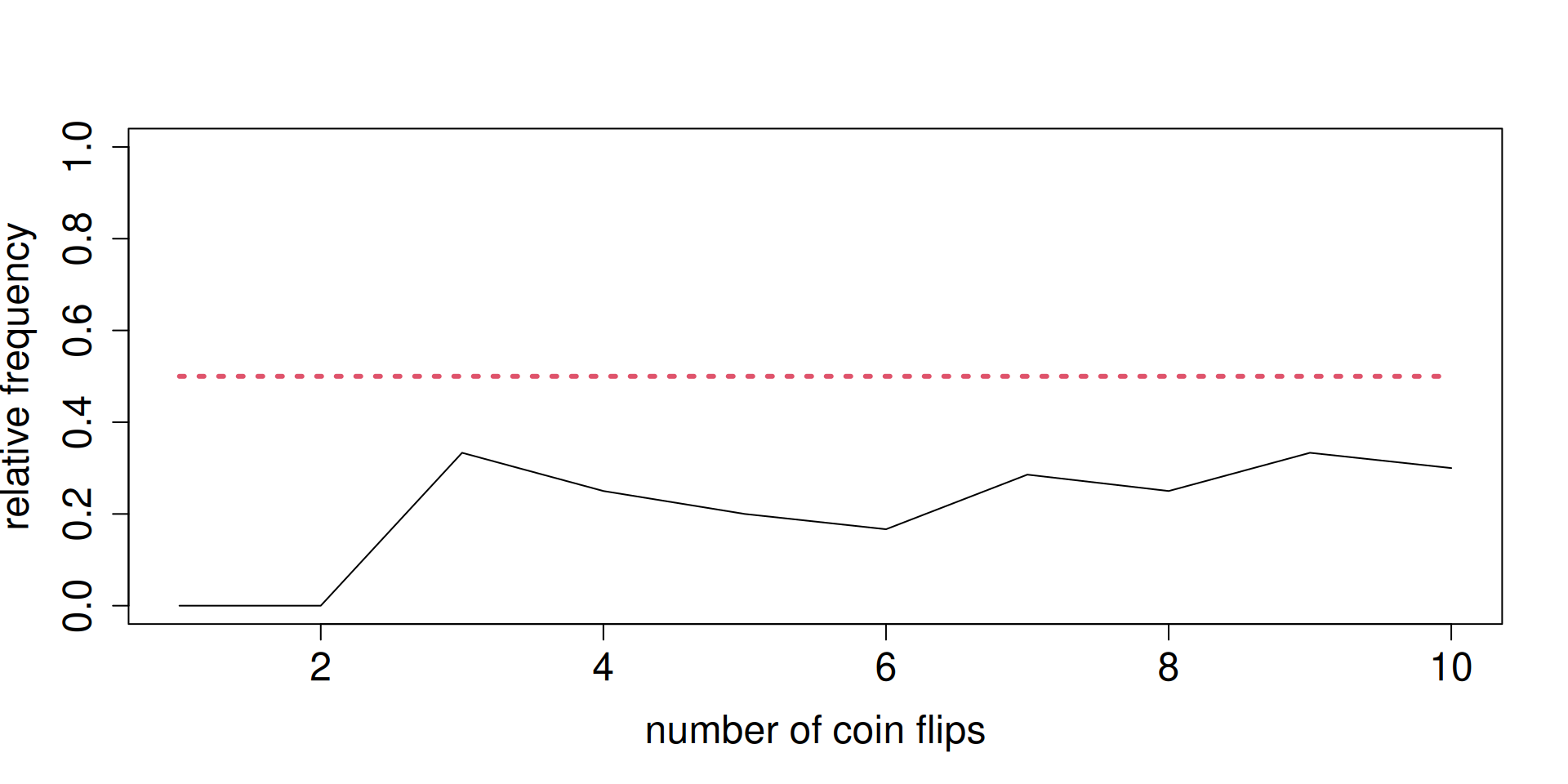
Pretend we are in the long run.
# Number of times to repeat the process of tossing a fair coin 10 times
nsim <- 2
# Repeat for nsim times "tossing of a fair coin 10 times"
a <- replicate(nsim, rbinom(10, 1, 0.5))
a
[,1] [,2]
[1,] 0 1
[2,] 0 1
[3,] 0 0
[4,] 0 1
[5,] 1 1
[6,] 1 1
[7,] 0 0
[8,] 1 1
[9,] 0 0
[10,] 0 1# Calculate the relative frequency or sample proportion for every repetition
props <- colMeans(a)
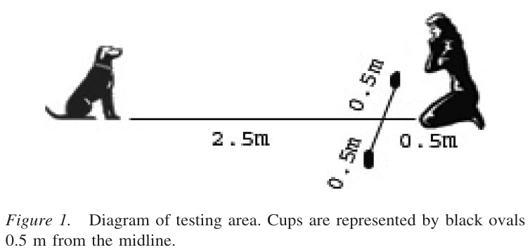
props[1] 0.3 0.7If you take the position that Harley cannot understand human gestures, how often can you hypothetically observe something more extreme than what you actually observed in real data?
In our case, it is given by 0.0123.
What decision will you make?
model, random, data generating process, long run, Monte Carlo simulation, fake-data simulation, law of large numbers, population, probability, relative frequency, expect, histogram, density, summary, hypothesis testing
| Informal | In general | In our example |
|---|---|---|
| Fixed constant of interest | Parameter | Population proportion |
| Data summary (can be hypothetical/fake or real) | Statistic | Sample proportion, relative frequency |