Lecture 5b

Digging deeper

Andrew Pua

2024-10-09

R commands related to the binomial

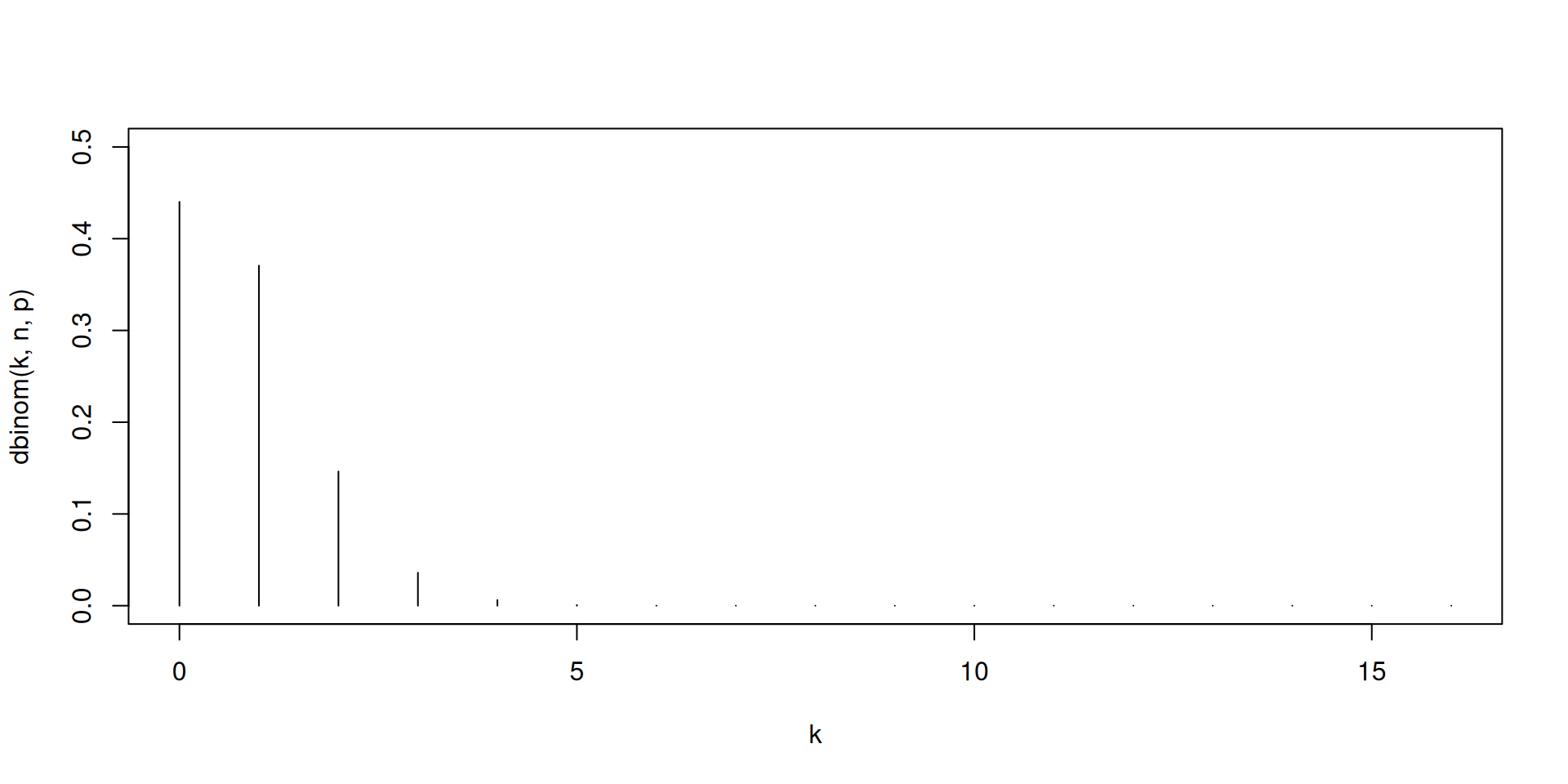
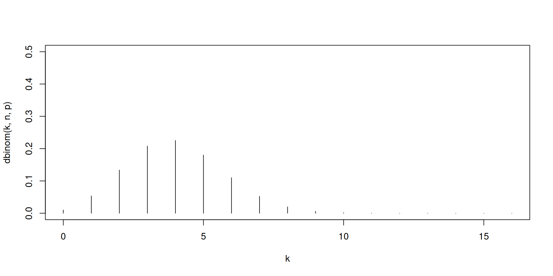
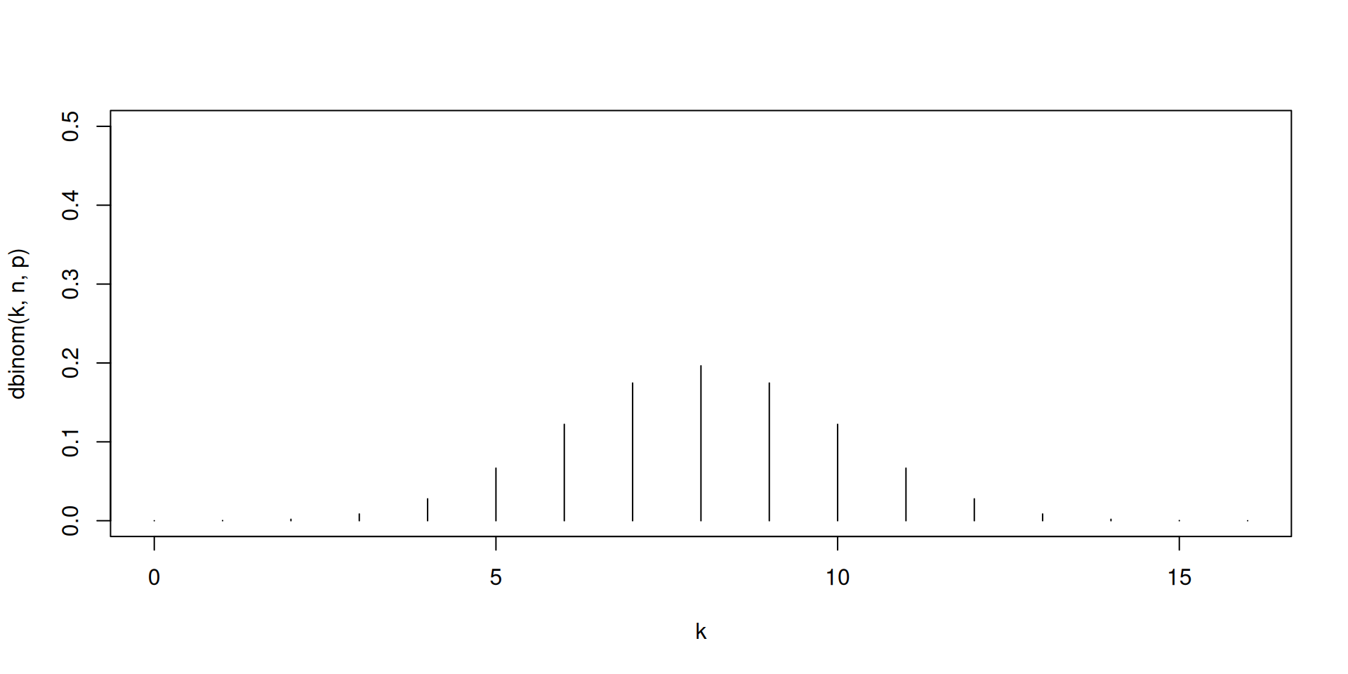
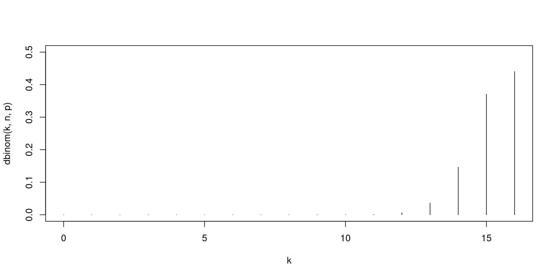
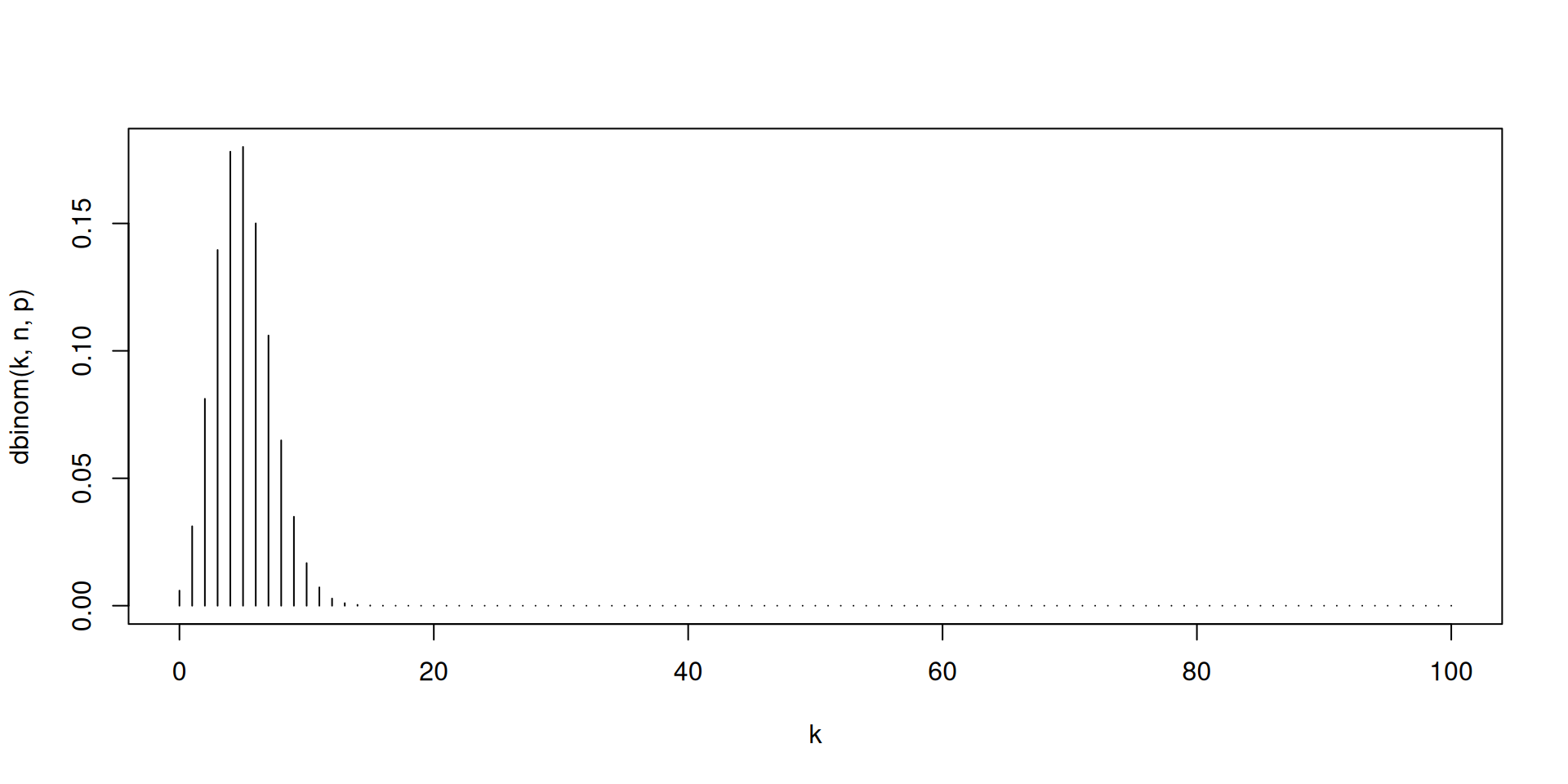
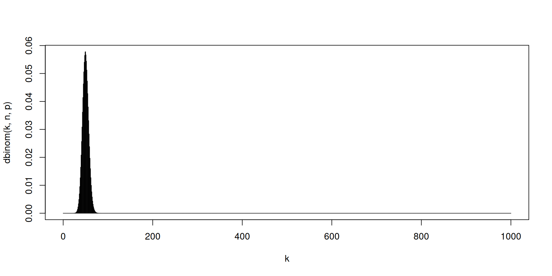
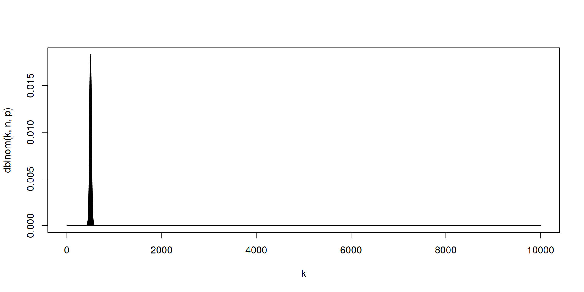
Suppose \(X\sim Bin\left(n,p\right)\). Let \(n\), \(p\), and \(k\) be given.

1. We use dbinom(k, n, p) to find \(\mathbb{P}\left(X=k\right)\).
2. We use pbinom(k, n, p, lower.tail = TRUE) to find \(\mathbb{P}\left(X\leq k\right)\).
3. If, in addition, we have to simulate nsim observations from \(X\), we use rbinom(nsim, n, p).

# Wasserman Example 1.10
1 - pbinom(0, 10, 0.5, lower.tail = TRUE)

[1] 0.9990234

# Alternative
pbinom(0, 10, 0.5, lower.tail = FALSE)

[1] 0.9990234

# Dekking et al Exercise 4.7b
# Probability that the batch contains no defective lamps 
dbinom(0, 1000, 0.001)

[1] 0.3676954

# Probability that the batch contains one defective lamp 
dbinom(1, 1000, 0.001)

[1] 0.3680635

# Probability that the batch contains more than two defective ones
1 - pbinom(2, 1000, 0.001)

[1] 0.08020934

# Alternatives
pbinom(2, 1000, 0.001, lower.tail = FALSE)

[1] 0.08020934

# Alternatives
1- (dbinom(0, 1000, 0.001) + dbinom(1, 1000, 0.001) + dbinom(2, 1000, 0.001))

[1] 0.08020934

Below you will find a function which can be used to plot what the binomial distribution looks like.

# Plotting binomial distributions
plot.binom <- function(n, p, ylim = NULL)
{
  k <- seq(0, n, 1)
  plot(k, dbinom(k, n, p), type = "h", ylim = ylim)
}

plot.binom(16, 0.05, ylim = c(0, 0.5))

plot.binom(16, 0.25, ylim = c(0, 0.5))

plot.binom(16, 0.5, ylim = c(0, 0.5))

plot.binom(16, 0.95, ylim = c(0, 0.5))

plot.binom(100, 0.05)

plot.binom(1000, 0.05)

plot.binom(10000, 0.05)

Discrete random variables

Definition 1 (Wasserman (2004, p. 22) Definition 2.9) \(X\) is discrete if it takes countably many values \(\{x_1 , x_2 , \ldots\}\). We define the probability function or probability mass function for \(X\) by \(f_X (x) = \mathbb{P}\left(X = x\right)\).

Definition 2 (Support) Let \(X\) be a random variable with probability mass function \(f_X\). The support of \(X\) is \[\mathsf{supp}\left(X\right)=\{x\in\mathbb{R}: f_X(x)> 0\}\]

1. Countable here means either finite or could be place in a one-to-one correspondence with the set of integers.

2. Not all functions could be probability mass functions. They have to satisfy

   1. \(f_X(x)\geq 0\) for any \(x\in\mathbb{R}\)
   2. \(\sum_i f_X(x_i) = 1\)

3. The cdf of \(X\) could be obtained as \[F_X(x)=\sum_{x_i\leq x} f_X(x_i)\]

4. Wasserman (2004, p. 21) Theorem 2.7: If the cdfs of two random variables \(X\) and \(Y\) are equal, then \(\mathbb{P}\left(X\in A\right)=\mathbb{P}\left(Y\in A\right)\).

5. If the cdfs of two random variables \(X\) and \(Y\) are equal, then \(X\) and \(Y\) are said to have identical distributions or equal in distribution.

6. Observe that it is not that the random variables \(X\) and \(Y\) are equal. Refer to Wasserman p. 25.

7. Not all functions could be cdfs. Refer to Wasserman (2004, p. 21) Theorem 2.8.

   • A cdf has to be an increasing function.
   • A cdf has to be bounded between 0 and 1.
   • \(F\) is right-continuous, i.e. \[F(x)=\lim_{y\to x,\ y>x} F(y).\]

8. What are the connections between the probability mass function and the cdf?

   • Think about how to recover one from the other.
   • Refer to Wasserman (2004, p. 24-25) Lemma 2.15.

Exercises to work on

1. Wasserman Chapter 2 Exercise 2
2. Dekking et al Chapter 4 Exercise 4.2
3. Dekking et al Chapter 4 Exercise 4.3
4. Dekking et al Chapter 4 Exercise 4.6