Lecture 5c
Summaries of distributions: Quantiles and expected values
2024-11-14
Quantile functions
Definition 1 (Wasserman (2004, p. 25) Definition 2.16) Let \(X\) be a random variable with cdf \(F\). The inverse cdf or quantile function is defined by \[F^{-1}\left(q\right)=\inf\{x: F(x)>q\}\] for \(q\in [0,1]\).
- \(F^{-1}(q)\) is called the \((100q)\)th percentile or the \(q\)-quantile.
You may see a slightly different definition in Evans and Rosenthal Definition 2.10.1. They have \[F^{-1}\left(q\right)=\min\{x: F(x)\geq q\}\] for \(q\in (0,1)\).
Quantile functions are used in everyday life:
- rankings
- for reporting risk measures
Should a firm introduce a new product?
A company wants to determine if they should enter a market. But there are other potential competitors. We have the following internal projections:
- Fixed costs of entering the market: 26 million
- Net present value of revenue minus variable costs in the whole market: 100 million
- Profits will depend on how many competitors enter the market. The 100 million will be shared equally among those in the market.
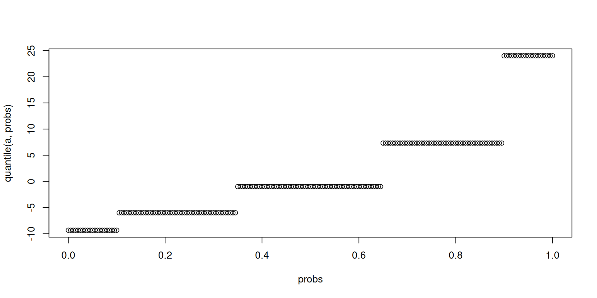
Let \(X\) be the number of other entrants in the market. This number is uncertain: \[\mathbb{P}\left(X=x\right)=\begin{cases}0.1 & \mathsf{if}\ x=1\\ 0.25 & \mathsf{if}\ x=2\\ 0.3 & \mathsf{if}\ x=3\\ 0.25 & \mathsf{if}\ x=4\\ 0.1 & \mathsf{if}\ x=5 \end{cases}\]
What would be the quantile function for the profit of the company? Derive it. Produce a simulation.
Expected value
Definition 2 (Wasserman (2004, p. 47) Definition 3.1) The expected value of a discrete random variable \(X\) is defined to be \[\mathbb{E}\left(X\right)=\sum_x xf_X(x)\] assuming that the sum is well-defined.
- Sometimes \(\mathbb{E}\left(X\right)\) is called the mathematical expectation, the population mean, or the first moment of \(X\).
There are also multiple acceptable notations: \(\mathbb{E}\left(X\right)\), \(\mathbb{E}X\), \(\mu\), \(\mu_X\).
The requirement of a well-defined expected value is not an issue if \(X\) takes on a finite number of values.
But it can be an issue if \(X\) takes on an infinite but countable number of values.
Illustrate using some exercises.
The expected value may not exist. Let \(k=\pm 1, \pm 2, \ldots\). Consider \[\mathbb{P}\left(X=k\right)=\frac{3}{\pi^2 k^2}.\]
Refer to other toy examples from Examples 3.1.10 and 3.1.11 of Evans and Rosenthal.
Another less artificial example is from the St. Petersburg paradox. Refer to Examples 3.1.12 and 3.1.13 of Evans and Rosenthal.
Three big reasons to study the expected value
- One criterion to decide which action to take when making decisions under uncertainty is to choose the action which produces the largest expected payoff.
- \(\mathbb{E}\left(X\right)\) is our “best” guess of what value \(X\) could take under a very specific criterion.
- The law of large numbers
Illustration of the law of large numbers
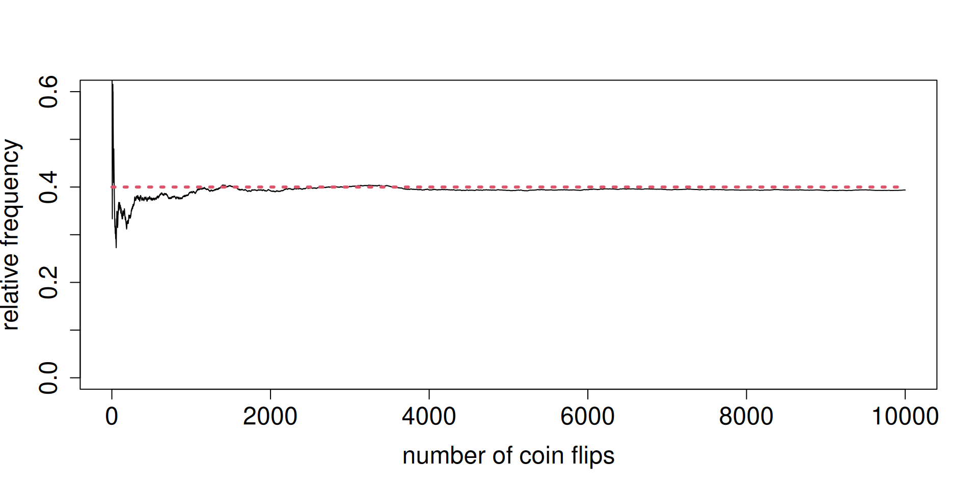
You already saw this in the context of tossing a coin. Let \(X=1\) if the toss produces heads and \(X=0\) if the toss produces tails. Then \[\mathbb{E}\left(X\right)=\mathbb{P}\left(X=1\right).\]
Set \(\mathbb{P}\left(X=1\right)=0.4\). Toss such a coin independently many times. Look at the relative frequency.
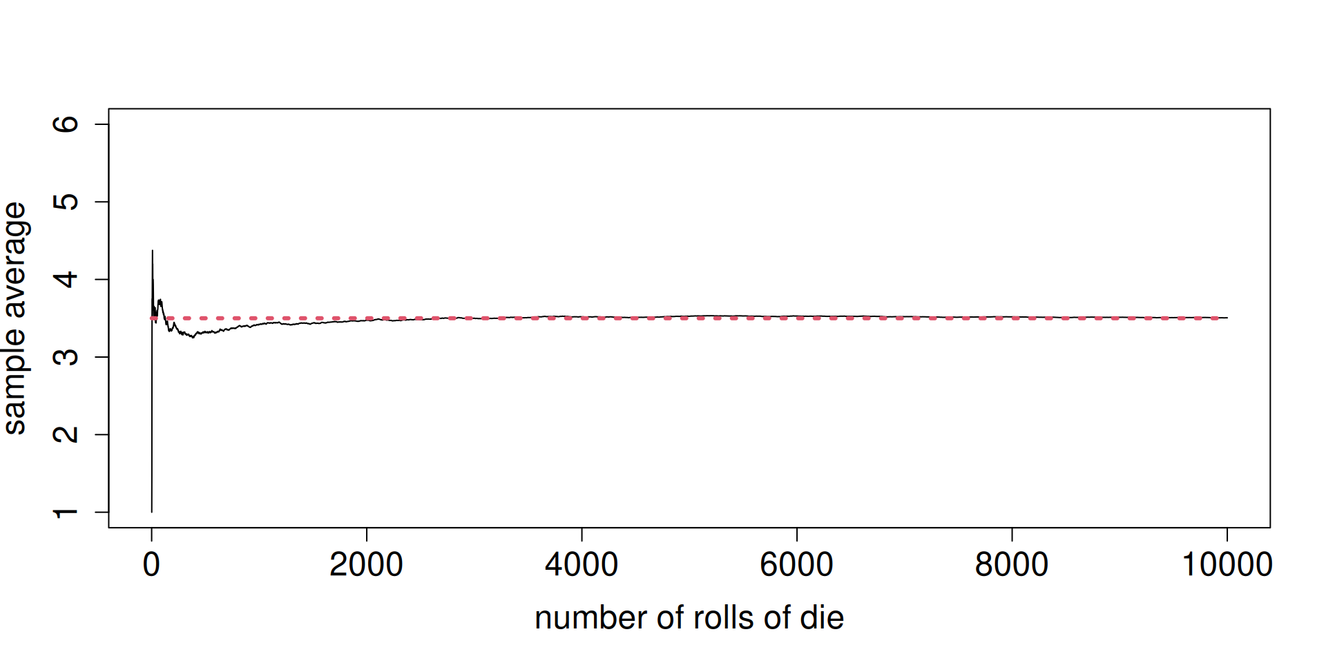
Now, roll a fair die. Let \(X\) be the outcome of one roll. Here, \(\mathbb{E}\left(X\right)=3.5\).
Instead of looking at a relative frequency, consider the sample mean of the outcomes from independently rolling a fair die as you have more and more rolls.
Notice the long-run order of the sample mean in the next slide.
Pay attention to the weighting scheme.
Notice in both cases, the expected value does NOT have to be one of the possible outcomes of \(X\).
The Rule of the Lazy Statistician
Refer to the distribution of \(X\) in Wasserman Chapter 2 Exercise 2.
- Find \(\mathbb{E}\left(X\right)\).
- Let \(Y=X^2\). Find \(\mathbb{E}\left(Y\right)\).
- Is it true that \(\mathbb{E}\left(X^2\right)\) and \(\left(\mathbb{E}\left(X\right)\right)^2\) are equal?
Wasserman (2004, p. 48) Theorem 3.6: Saves us time in computing expected values of functions of some random variable \(X\).
Some very useful properties of expected values:
- Let \(X\) be a random variable. Let \(a\) and \(b\) be constants. \[\mathbb{E}\left(aX+b\right)=a\mathbb{E}\left(X\right)+b.\]
- Wasserman (2004, p. 63) Theorem 4.1 on Markov’s inequality: Existence of the expected value creates constraints on the tails of the distribution.
- Wasserman (2004, p. 66) Theorem 4.9 on Jensen’s inequality: If \(g\) is convex, then \[\mathbb{E}\left(g(X)\right) \geq g\left(\mathbb{E}\left(X\right)\right).\]
Moments
Definition 3 (Wasserman (2004, p. 47)) The \(k\)th moment of \(X\) is defined to be \(\mathbb{E}\left(X^k\right)\) assuming that \(\mathbb{E}\left(|X|^k\right)<\infty\).
- Wasserman (2004, p. 49) Theorem 3.10: If \(\mathbb{E}\left(X^k\right)\) exists and if \(j<k\), then \(\mathbb{E}\left(X^j\right)\) exists.
- May not appear to have practical relevance, but has consequences for risk management settings
Variance
Definition 4 (Wasserman (2004, p. 51)) Let \(X\) be a random variable with mean \(\mu\). The variance of \(X\), denoted by \(\sigma^2\), \(\sigma^2_X\), \(\mathbb{V}\left(X\right)\), \(\mathbb{V}X\), or \(\mathsf{Var}\left(X\right)\) is defined \[\sigma^2=\mathbb{E}\left(X-\mu\right)^2,\] assuming that this expectation exists. The standard deviation is \(\mathsf{sd}(X)=\sqrt{\mathbb{V}\left(X\right)}\) and is also denoted by \(\sigma\) or \(\sigma_X\).
Illustrate using examples.
Wasserman (2004, p. 51) Theorem 3.15 points to two important properties of the variance:
- A computational shortcut: \[\mathsf{Var}\left(X\right)=\mathbb{E}\left(X^2\right)-\mu^2\]
- Let \(X\) be a random variable. Let \(a\) and \(b\) be constants. Then, \[\mathsf{Var}\left(aX+b\right)=a^2\mathsf{Var}\left(X\right).\]
- Where did the name standard deviation come from? The answer lies in Wasserman (2004, p. 64) Theorem 4.2 on Chebyshev’s inequality.
Theorem 1 (Wasserman (2004, p. 64) Chebyshev’s inequality) Let \(\mu=\mathbb{E}\left(X\right)\) and \(\sigma^2=\mathsf{Var}\left(X\right)\). Then, for all \(t>0\), \[\mathbb{P}\left(|X-\mu|\geq t\right) \leq \frac{\sigma^2}{t^ 2}.\]
If we let \(Z=\dfrac{X-\mu}{\sigma}\), then \[\mathbb{P}\left(|Z|\geq k\right)\leq \frac{1}{k^2}.\]
\(Z=\dfrac{X-\mu}{\sigma}\) is called standardization.
Therefore, we know a lot about the tail behavior of a standardized random variable! In particular, \[\mathbb{P}\left(|Z|\geq 2\right)\leq \frac{1}{4}, \ \ \mathbb{P}\left(|Z|\geq 3\right)\leq \frac{1}{9}\]