Lecture 6a

The building blocks of statistical inference

Andrew Pua

2024-11-21

What is statistical inference?

1. One of the things that statisticians do is statistical inference.

   1. In computer science, statistical inference is called learning.
   2. Inference is the process of using data to infer the distribution that generated the data.

2. We are usually blessed with only one dataset. We think of it as being drawn from some data generating process.

3. We want to infer either the entire data generating process or features of the data generating process using only one dataset.

4. We are actually reversing the process you have been seeing in our discussions of probability and random variables.

5. There are three major types of inference:

   1. Point estimation, e.g. the sample mean as a way to learn \(\mu\)
   2. Confidence sets, e.g., finite sample confidence intervals using Chebyshev’s inequality
   3. Hypothesis testing, e.g. introduced immediately in the first three weeks of the course

6. Slightly more specific:

   1. Point estimation: Providing a best guess of some unknown quantity of interest – could be a parameter or an entire function
   2. Confidence sets: Providing a “range” of values which “trap” some unknown quantity of interest with a pre-specified probability
   3. Hypothesis testing: Start with some default theory, called the null hypothesis, and ask if the data provide sufficient evidence to reject the theory. If not, retain the null hypothesis.

What you have so far

1. The sample mean \(\overline{X}_n\) is used as a point estimator of \(\mu\).
2. We constructed a finite-sample confidence interval for \(\mu\) using Chebyshev’s inequality.
3. In the IID Bernoulli case, \(\mu\) is equal to the probability of success. We have tested the null that the probability of success is equal to some pre-specified value.

4. But these are extremely limited and there are unanswered questions.

   1. Sometimes we may not necessarily be just interested in \(\mu\).
   2. The guarantee provided by Chebyshev’s inequality can be conservative.
   3. Why are hypothesis tests designed the way they are?
   4. What happens when sample sizes are large?

Effects of increasing sample size on the sampling distribution of \(\overline{X}_n\)

1. Recall the example where \(X\) is a random variable whose distribution is \(\mathbb{P}\left(X=2\right)=1/10\), \(\mathbb{P}\left(X=3\right)=1/10\), \(\mathbb{P}\left(X=5\right)=8/10\).
2. Obtain \(n\) IID draws from this distribution.
3. Display the histogram for the sampling distribution of the sample mean.
4. What do you notice as \(n\to\infty\)?

a <- replicate(10^4, sample(c(2, 3, 5), 2, prob = c(0.1, 0.1, 0.8), replace = TRUE))
sample.means <- colMeans(a)
hist(sample.means, cex.axis = 1.5, cex.lab = 1.5, main = "")

a <- replicate(10^4, sample(c(2, 3, 5), 2, prob = c(0.1, 0.1, 0.8), replace = TRUE))
sample.means <- colMeans(a)
hist(sample.means, cex.axis = 1.5, cex.lab = 1.5, main = "")

a <- replicate(10^4, sample(c(2, 3, 5), 4, prob = c(0.1, 0.1, 0.8), replace = TRUE))
sample.means <- colMeans(a)
hist(sample.means, cex.axis = 1.5, cex.lab = 1.5, main = "", xlim = c(2,5))

a <- replicate(10^4, sample(c(2, 3, 5), 8, prob = c(0.1, 0.1, 0.8), replace = TRUE))
sample.means <- colMeans(a)
hist(sample.means, cex.axis = 1.5, cex.lab = 1.5, main = "", xlim = c(2,5))

a <- replicate(10^4, sample(c(2, 3, 5), 16, prob = c(0.1, 0.1, 0.8), replace = TRUE))
sample.means <- colMeans(a)
hist(sample.means, cex.axis = 1.5, cex.lab = 1.5, main = "", xlim = c(2,5))

a <- replicate(10^4, sample(c(2, 3, 5), 64, prob = c(0.1, 0.1, 0.8), replace = TRUE))
sample.means <- colMeans(a)
hist(sample.means, cex.axis = 1.5, cex.lab = 1.5, main = "", xlim = c(2,5))

a <- replicate(10^4, sample(c(2, 3, 5), 128, prob = c(0.1, 0.1, 0.8), replace = TRUE))
sample.means <- colMeans(a)
hist(sample.means, cex.axis = 1.5, cex.lab = 1.5, main = "", xlim = c(2,5))

a <- replicate(10^4, sample(c(2, 3, 5), 256, prob = c(0.1, 0.1, 0.8), replace = TRUE))
sample.means <- colMeans(a)
hist(sample.means, cex.axis = 1.5, cex.lab = 1.5, main = "", xlim = c(2,5))

a <- replicate(10^4, sample(c(2, 3, 5), 512, prob = c(0.1, 0.1, 0.8), replace = TRUE))
sample.means <- colMeans(a)
hist(sample.means, cex.axis = 1.5, cex.lab = 1.5, main = "", xlim = c(2,5))

a <- replicate(10^4, sample(c(2, 3, 5), 1024, prob = c(0.1, 0.1, 0.8), replace = TRUE))
sample.means <- colMeans(a)
hist(sample.means, cex.axis = 1.5, cex.lab = 1.5, main = "", xlim = c(2,5))

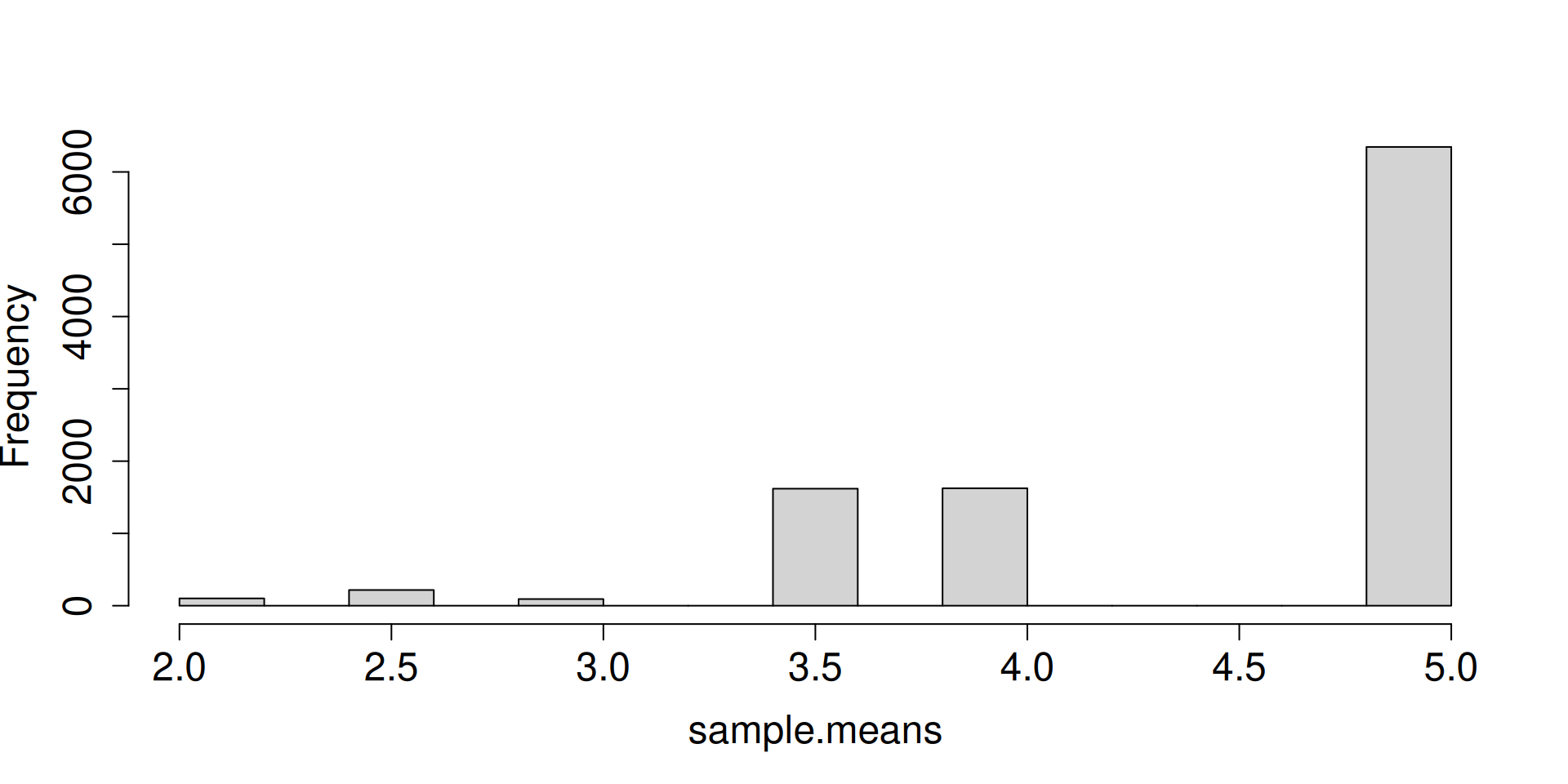
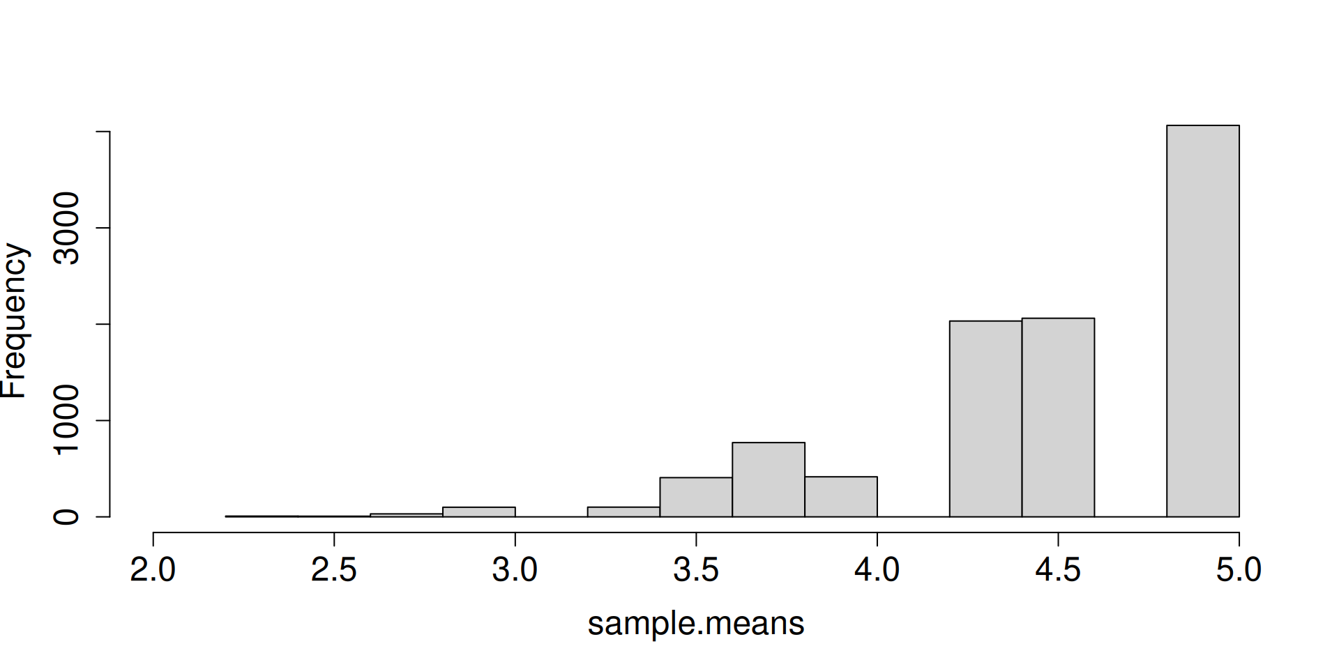
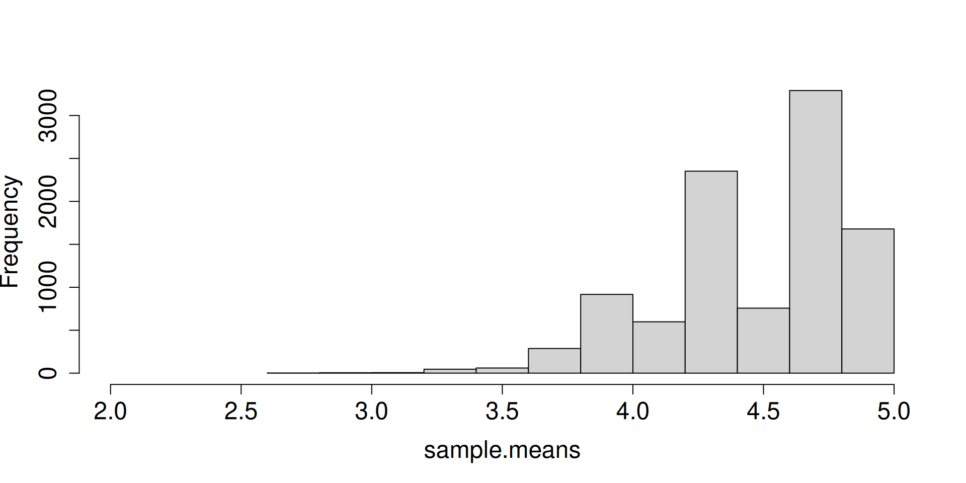
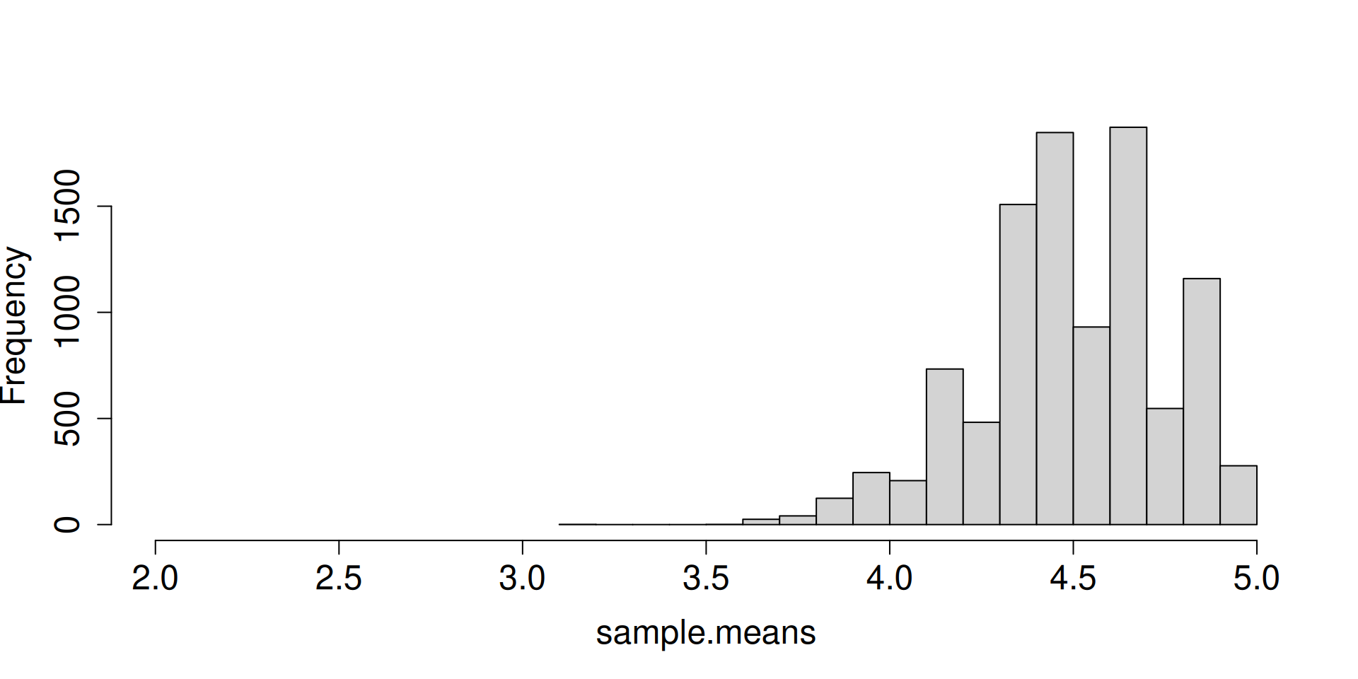
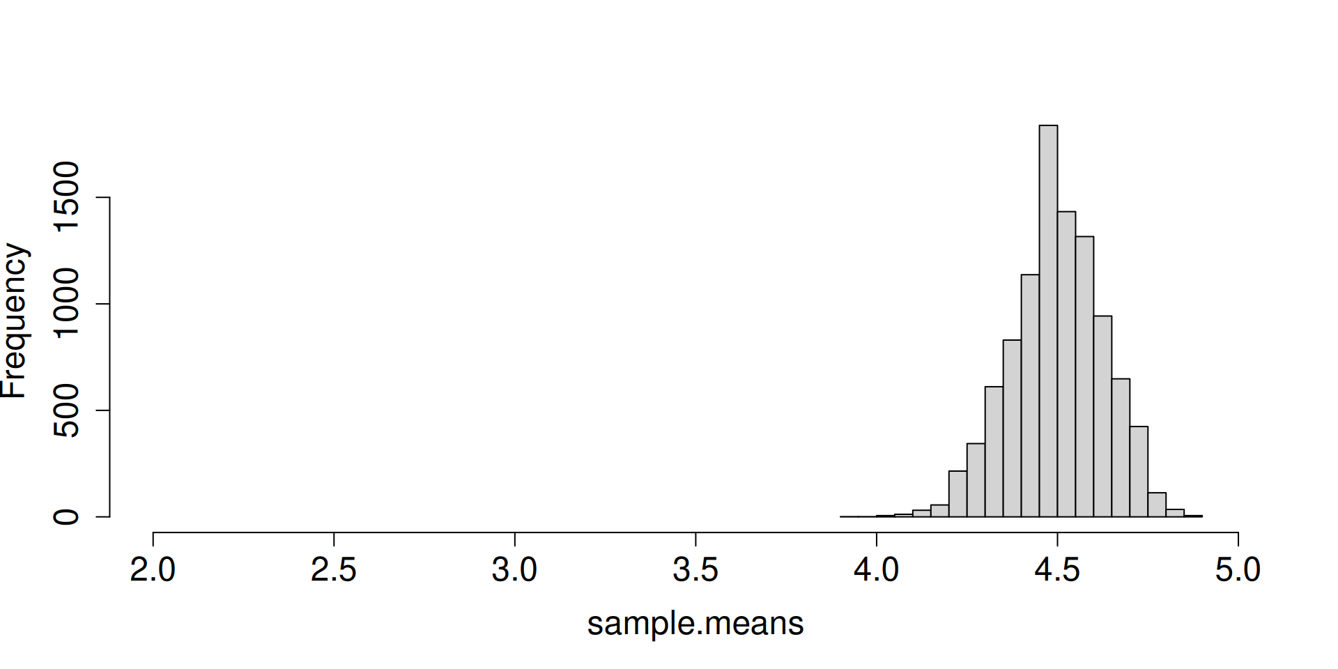
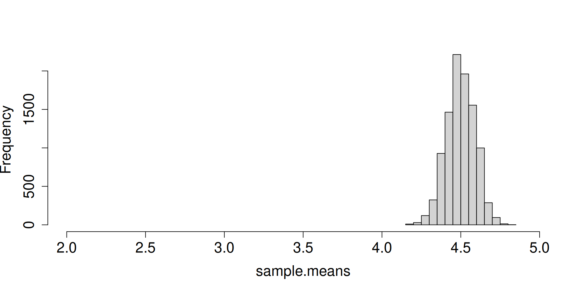
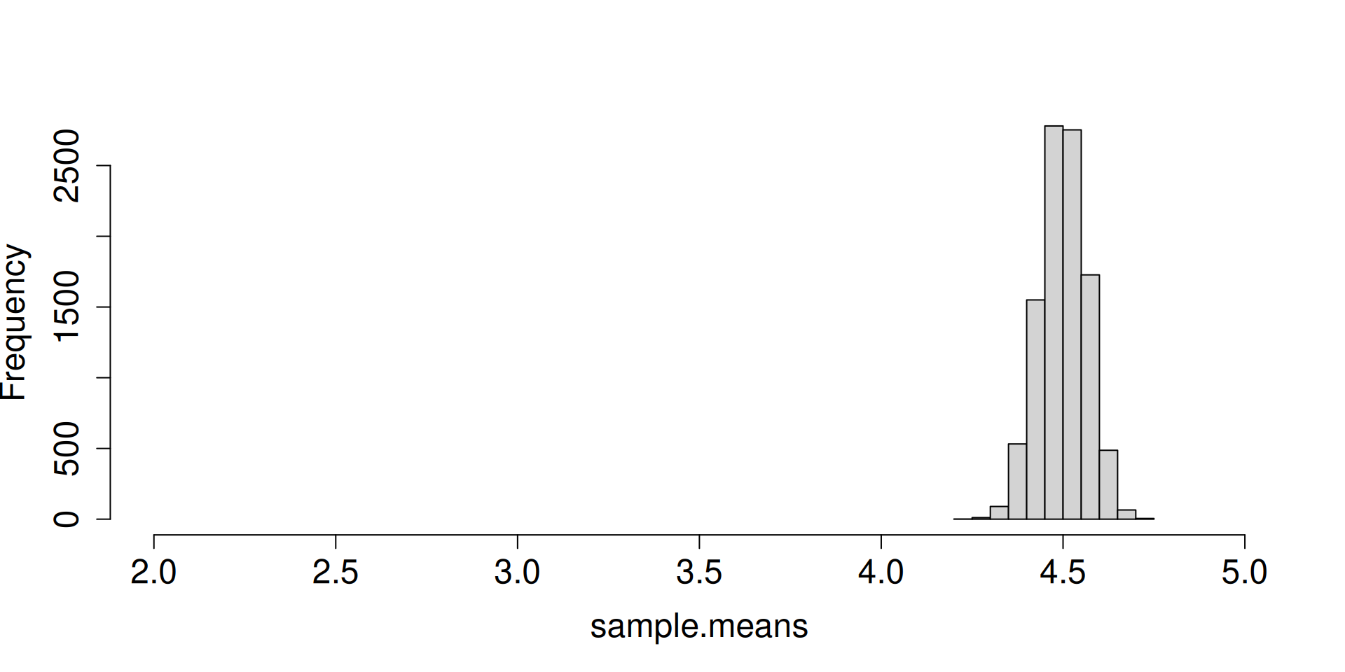
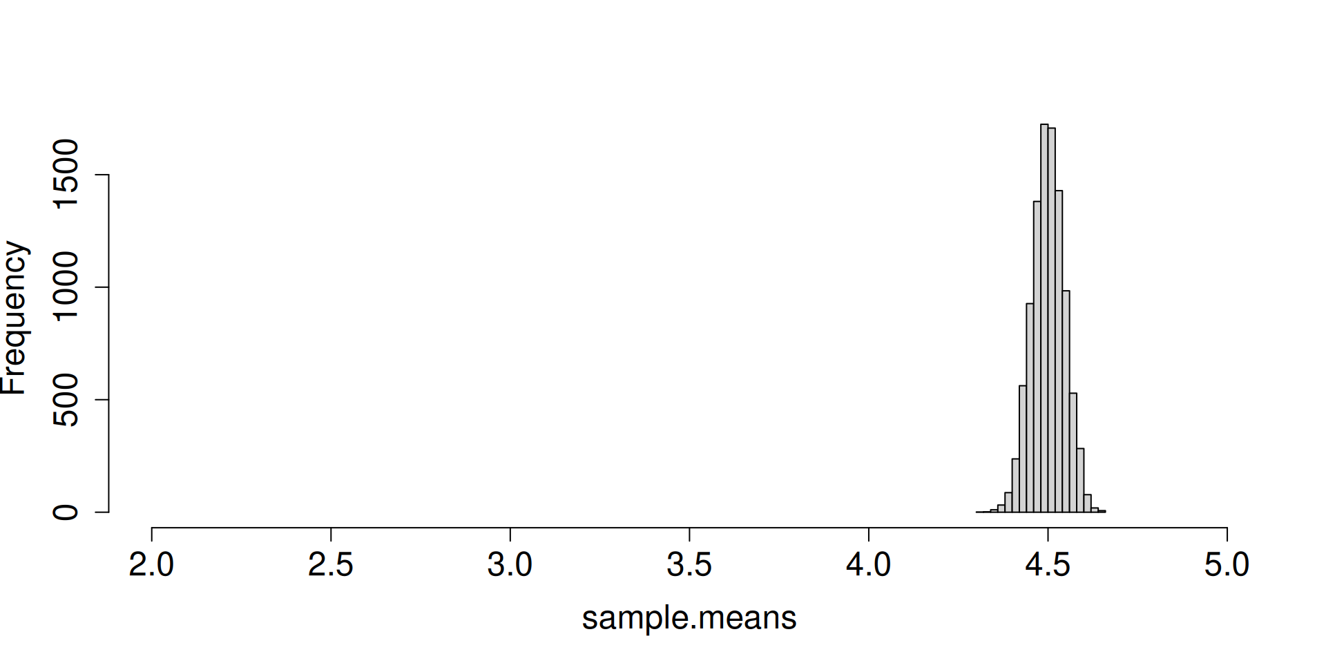
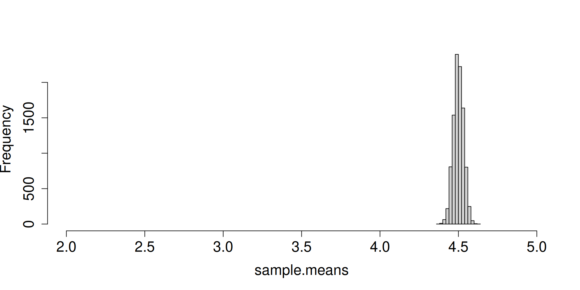
5. This is really the perfect time to create your own R function (we have seen this many times). You can create histograms, but here I focus on the mean, variance, and standard deviation of the sampling distribution of the sample mean.

dist.mean <- function(n)
{
  a <- replicate(10^4, sample(c(2, 3, 5), n, prob = c(0.1, 0.1, 0.8), replace = TRUE))
  sample.means <- colMeans(a)
  return(c(mean(sample.means), var(sample.means), sd(sample.means)))
}

6. Allow \(n\) to be the input and let it increase in size.

sapply(2^(1:10), dist.mean)

      [,1]  [,2]  [,3]   [,4]   [,5]   [,6]    [,7]   [,8]    [,9]   [,10]
[1,] 4.490 4.497 4.494 4.4999 4.5012 4.4986 4.49988 4.5001 4.50031 4.49988
[2,] 0.538 0.264 0.134 0.0638 0.0329 0.0167 0.00811 0.0041 0.00199 0.00105
[3,] 0.733 0.514 0.365 0.2526 0.1812 0.1294 0.09007 0.0640 0.04464 0.03244

1.05/(2^(1:10))

 [1] 0.52500 0.26250 0.13125 0.06563 0.03281 0.01641 0.00820 0.00410 0.00205
[10] 0.00103

1.05/sqrt((2^(1:10)))

 [1] 0.7425 0.5250 0.3712 0.2625 0.1856 0.1313 0.0928 0.0656 0.0464 0.0328

6. What are the forces at work here? Distribution is getting more and more concentrated at \(\mu\). There seems to be an emerging shape for the distribution as well.

Concentration of the sampling distribution of the sample mean

Theorem 1 (The Weak Law of Large Numbers) If \(X_1, \ldots, X_n\) are IID random variables with mean \(\mathbb{E}(X_i)=\mu\) and \(\mathsf{Var}\left(X_i\right)=\sigma^2\), then for all \(\varepsilon>0\), \[\lim_{n\to\infty} \mathbb{P}\left(|\overline{X}_n-\mu|\geq \varepsilon\right)= 0.\]

1. You have already seen the law of large numbers at work so many times in the course.
2. An argument based on Chebyshev’s inequality was also presented in Lecture 5d.
3. Wasserman (2004, p. 76, Theorem 5.6) actually states the theorem without \(\mathsf{Var}\left(X_i\right)=\sigma^2\), but the proof will no longer be based on Chebyshev’s inequality.
4. Another way to write the conclusion of the theorem is \[\overline{X}_n\overset{p}{\to} \mu.\]

5. \(\overline{X}_n\overset{p}{\to} \mu\) is usually expressed in many ways. As \(n\to \infty\),

   1. A law of large numbers applies to \(\overline{X}_n\).
   2. \(\overline{X}_n\) is a consistent estimator of \(\mu\). Refer to Definition 6.7 of Wasserman (2004), p. 90.
   3. The sequence \(\overline{X}_1, \overline{X}_2, \ldots\) converges in probability to \(\mu\).

6. Take note that \(\mu=\mathbb{E}\left(X_i\right)\), the common mean of the marginal distributions of \(X_1,X_2, ,\ldots\).

The emerging shape of the distribution

1. Standardize first in order to “counter” two things:

   1. the effect of the distribution “moving” from left to right
   2. the effect of the distribution of the sample mean concentrating at \(\mu\).

2. Here we know that \(\mathbb{E}\left(\overline{X}_n\right)=\mu\) and \(\mathsf{Var}\left(\overline{X}_n\right)=\sigma^2/n\).

3. Plot the distribution of the standardized sample mean \(\dfrac{\overline{X}_n-\mu}{\sigma/\sqrt{n}}\) instead.

4. We know \(\mu\) and \(\sigma^2\) for the purposes of the simulation. In practice, we do not know them (otherwise, what is the point of a statistics course?).

plot.dist.mean <- function(n)
{
  a <- replicate(10^4, sample(c(2, 3, 5), n, prob = c(0.1, 0.1, 0.8), replace = TRUE))
  st.sample.means <- (colMeans(a)-4.5)/(sqrt(1.05/n))
  par(mfrow = c(1, 2))
  hist(st.sample.means, cex.axis = 1.5, cex.lab = 1.5, main = "", xlim = c(-4,4))
  plot(ecdf(st.sample.means))
  curve(pnorm, add=TRUE, col="red")
}

plot.dist.mean(2)

plot.dist.mean(4)

plot.dist.mean(8)

plot.dist.mean(16)

plot.dist.mean(32)

plot.dist.mean(64)

plot.dist.mean(128)

plot.dist.mean(256)

plot.dist.mean(512)

plot.dist.mean(1024)

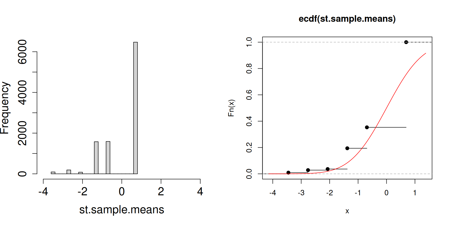
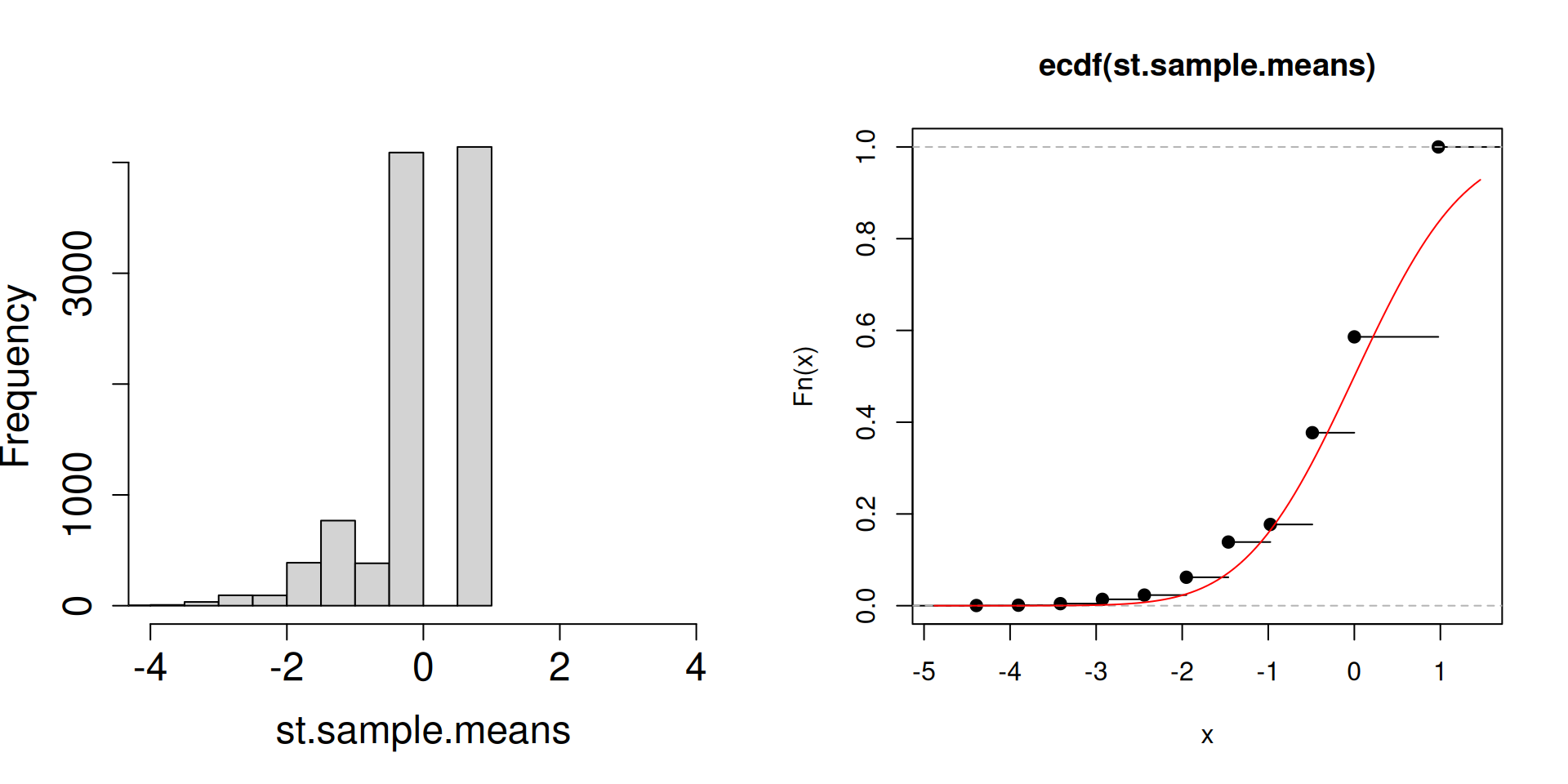
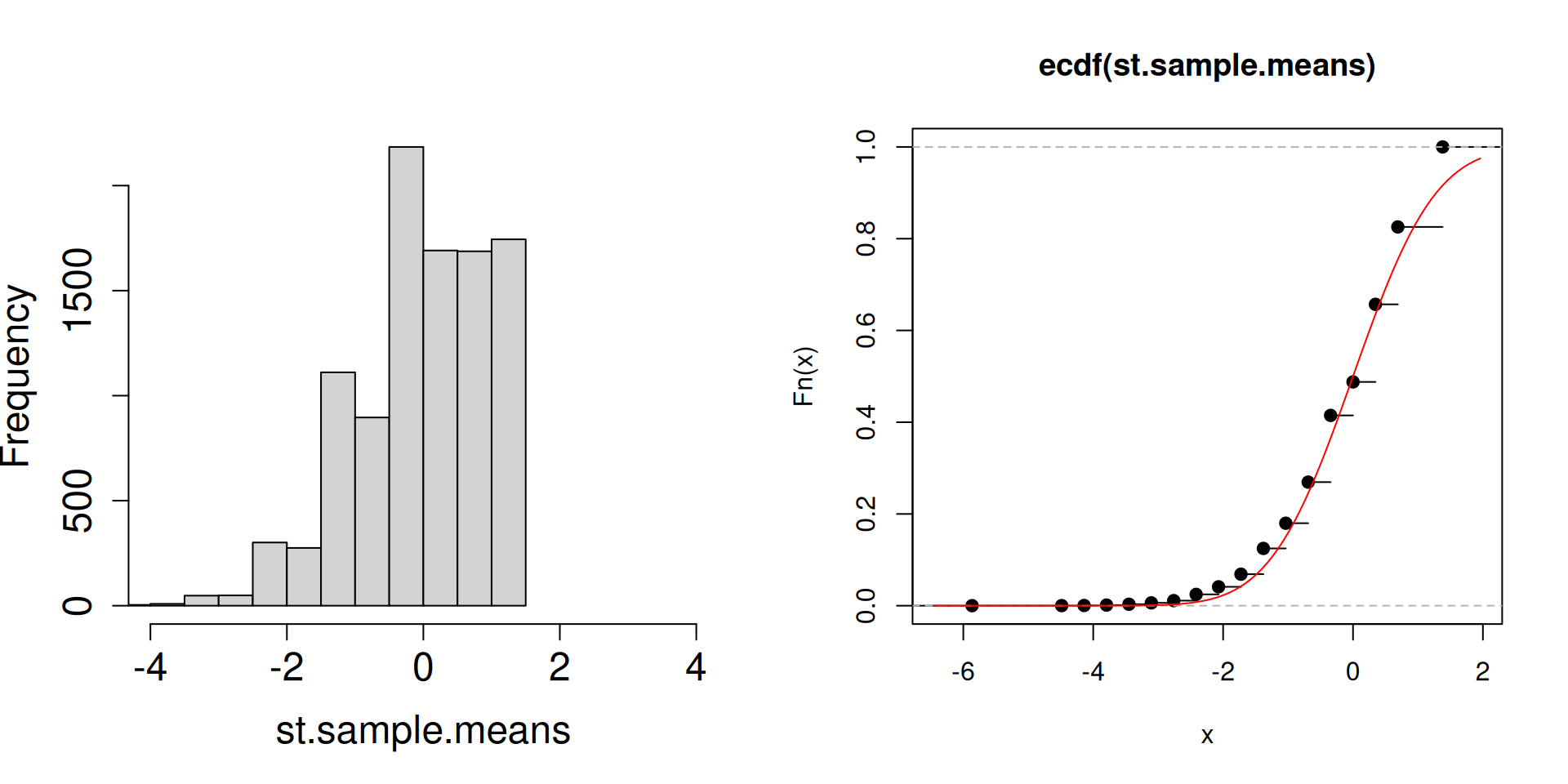
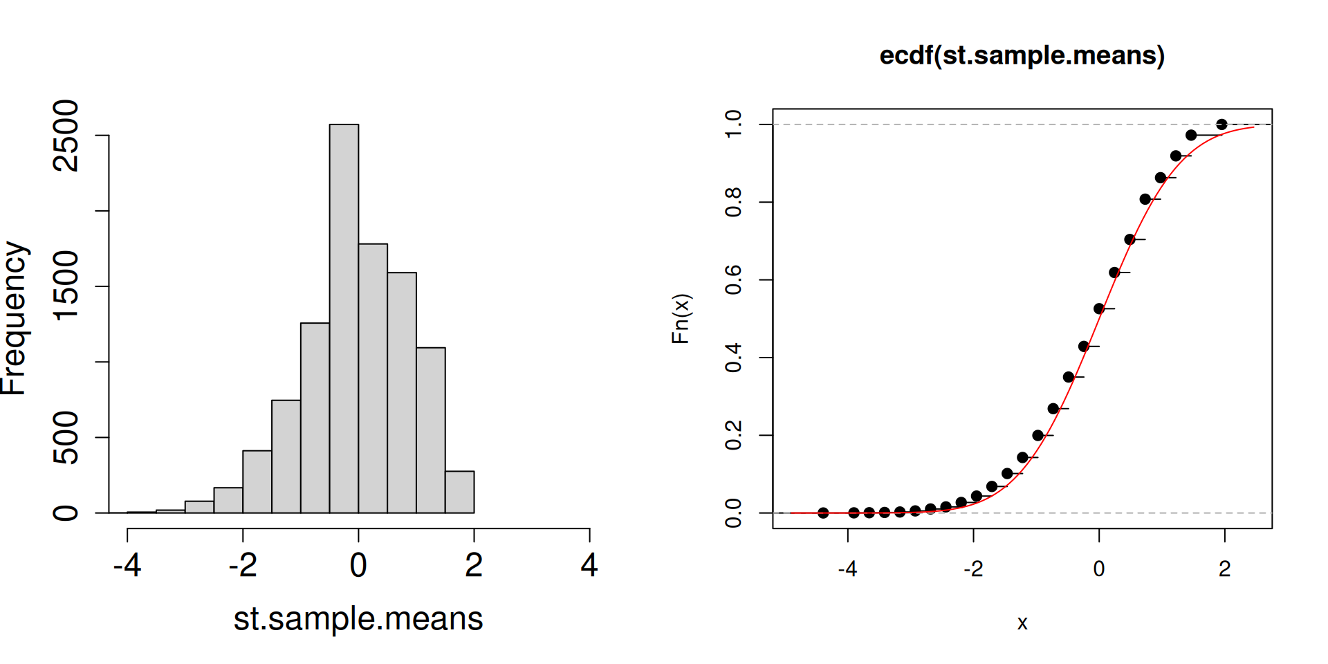
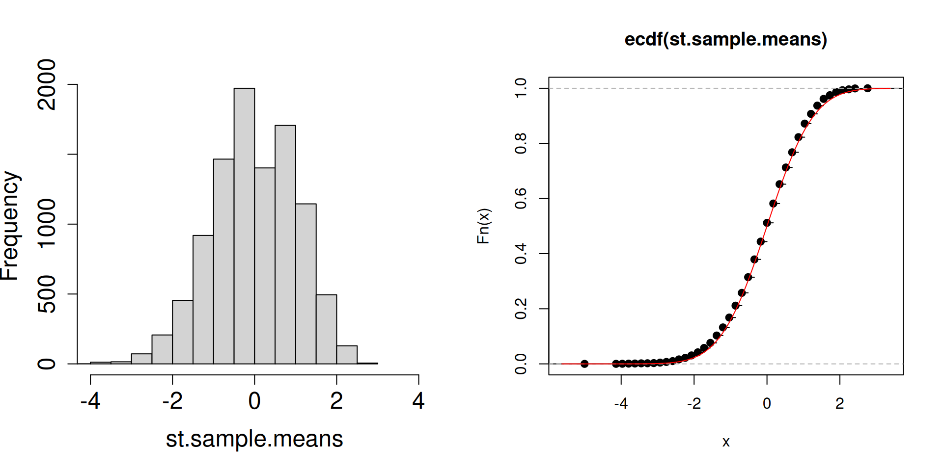
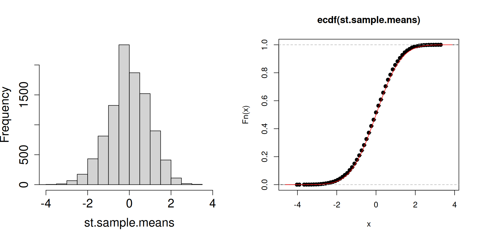
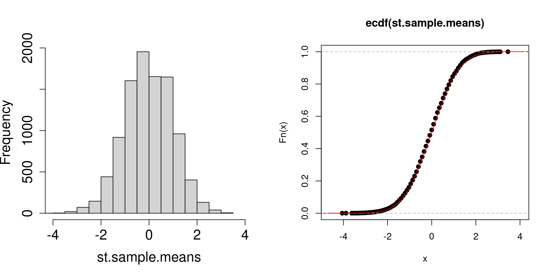
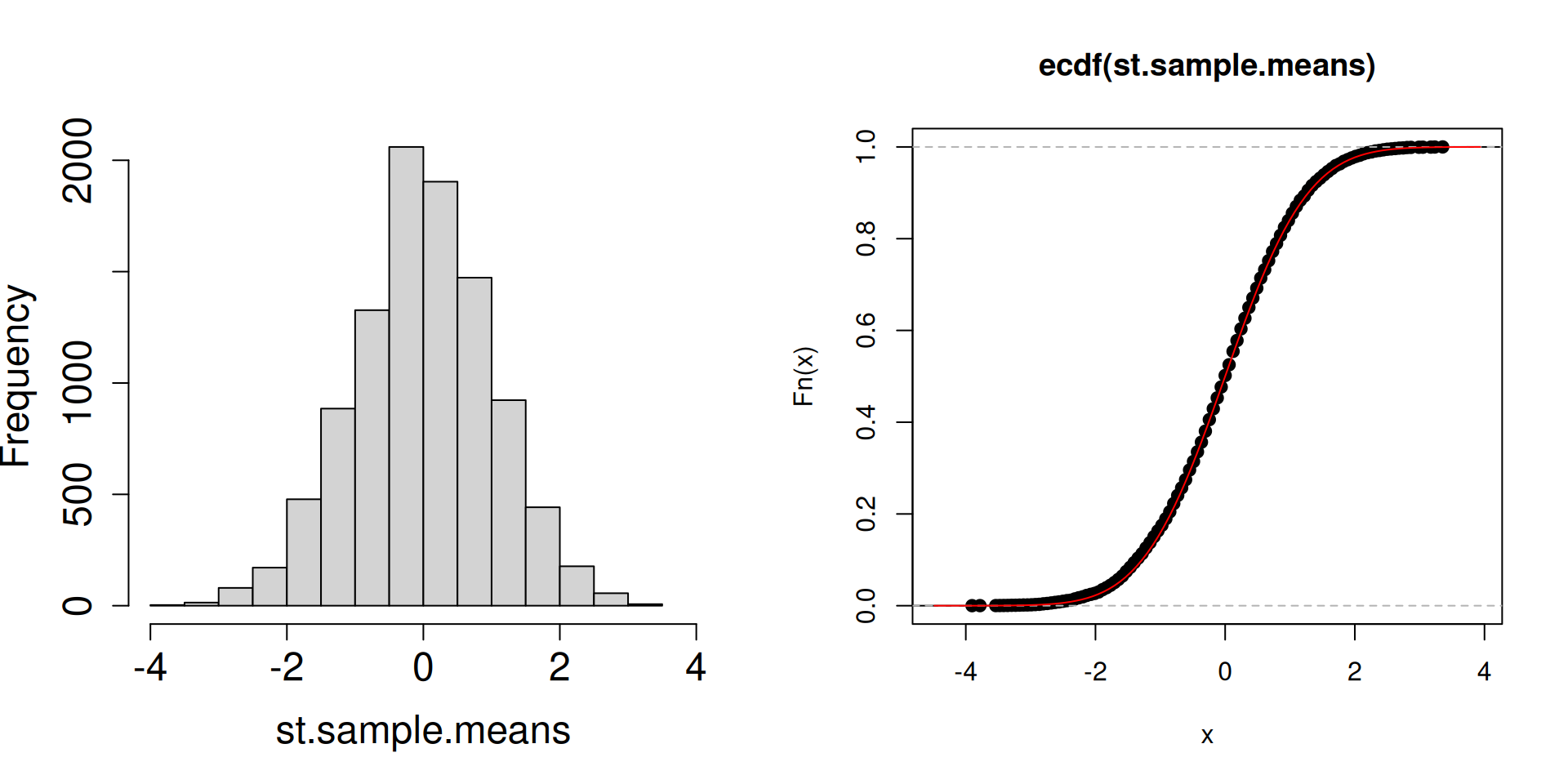
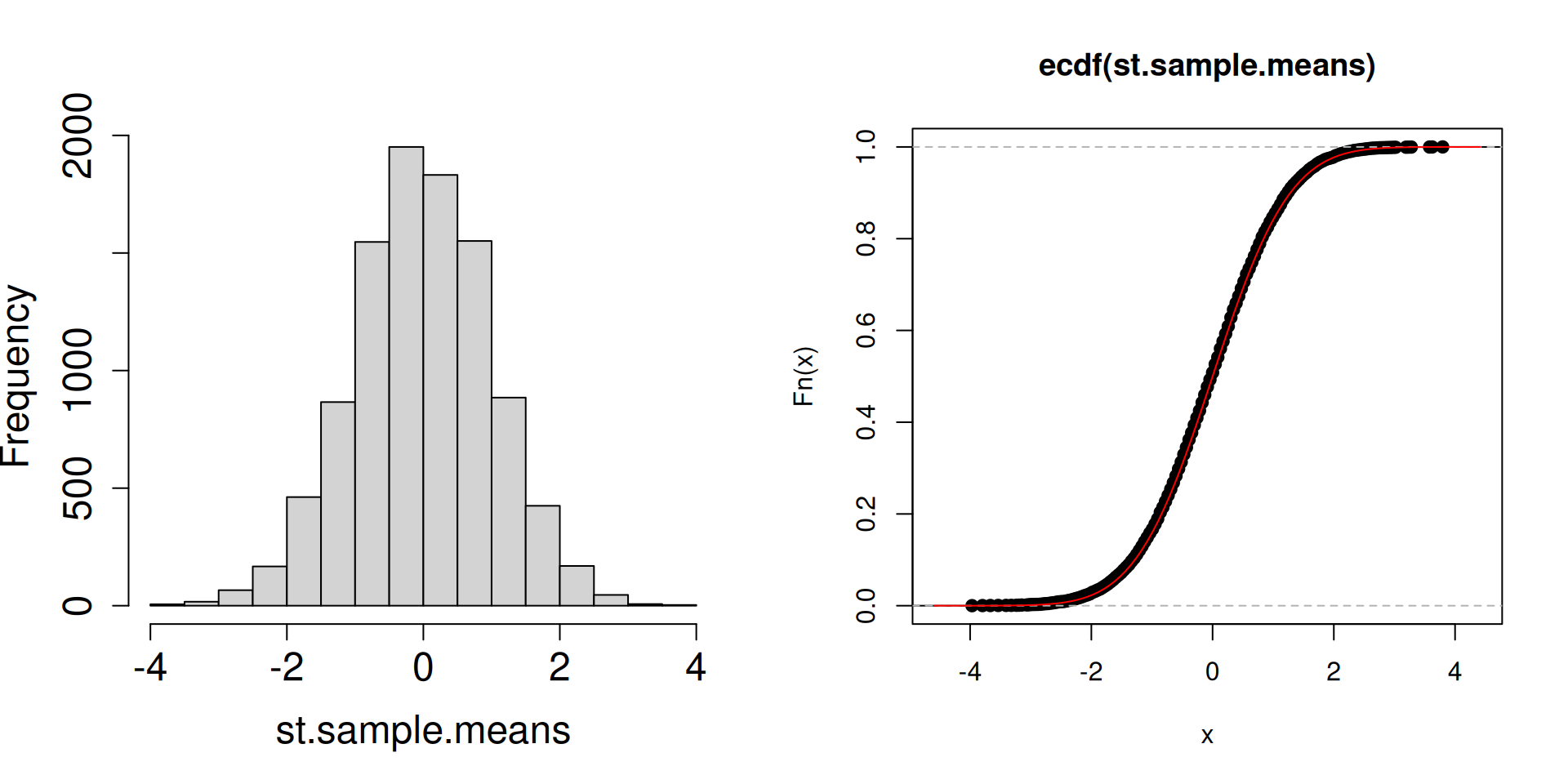
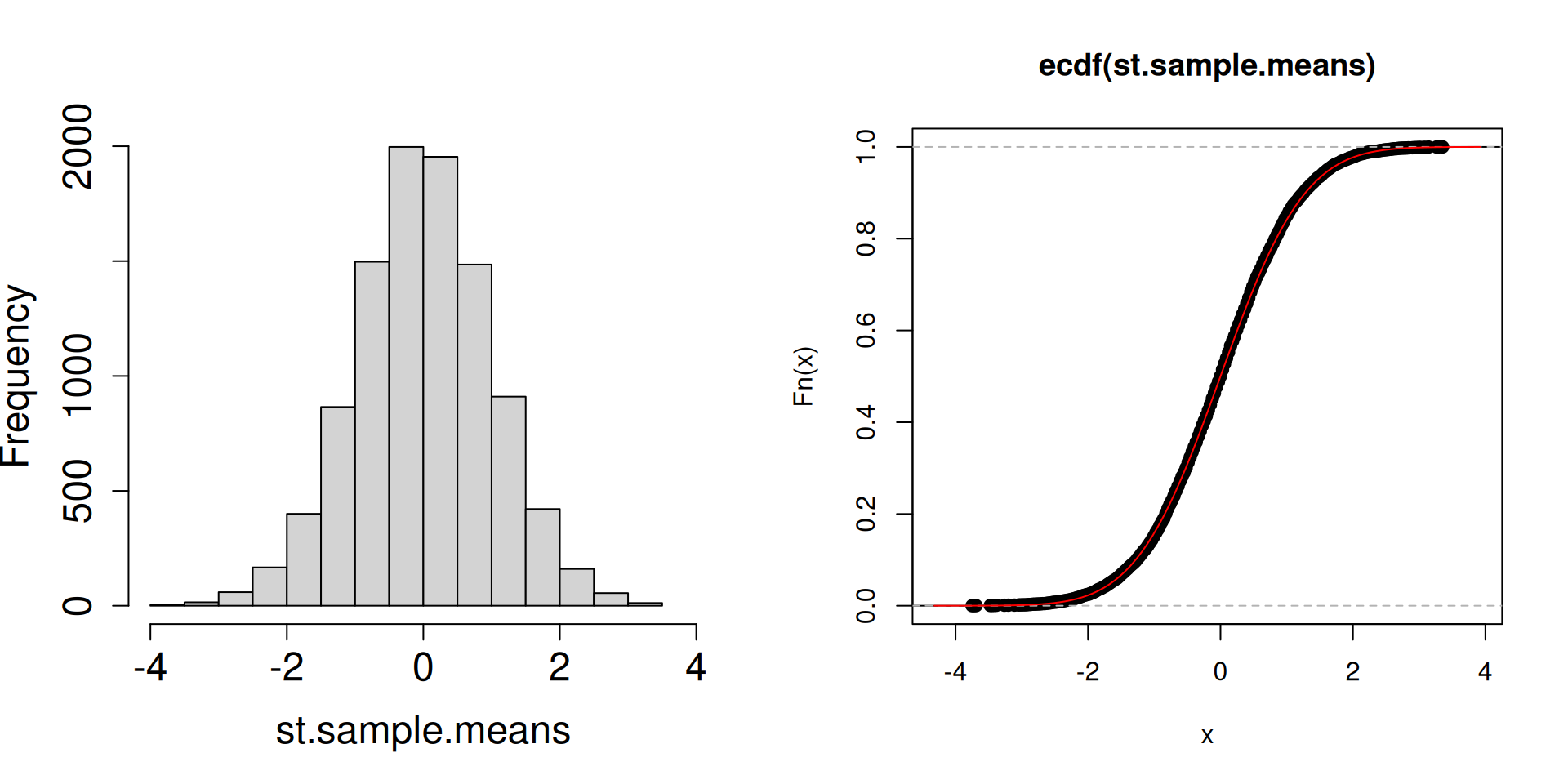
What is the red curve?

1. The red curve is actually the cdf of a random variable \(Z\) that has a standard normal distribution (another special distribution). The standard normal cdf is usually written at \(\Phi(z)\) has the following form: \[\Phi(z)=\mathbb{P}\left(Z\leq z\right)=\int_{-\infty}^z \frac{1}{\sqrt{2\pi}}\exp\left(-\frac{1}{2}x^2\right)\, dz.\]

2. This is probably one of the more famous continuous distributions.

3. Compared to the cdfs of discrete random variables you have seen so far, the red curve looks very different. In particular, there are no jumps.

4. What matters is that the cdf of a standard normal random variable is a good approximation of the cdf of the sampling distribution of the standardized sample mean.

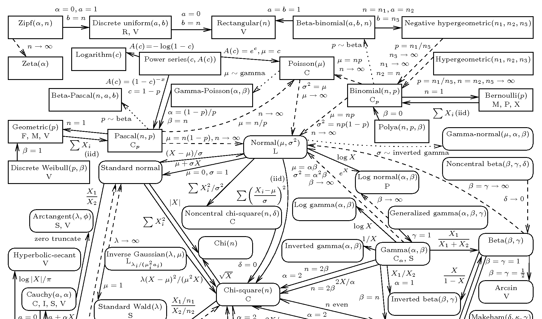
5. We will just take a small dip into continuous random variables.

Digression: Continuous random variables

In the slides, pay attention to whether the word “discrete” was specified or not. Differences compared to discrete random variables:

1. Probability density functions (pdf) versus probability mass functions (pmf)

   1. Heights of those functions differ in meaning: for the pdf it would be density, for the pmf it would be probability
   2. Heights of a pdf can exceed 1.

2. Cdf is continuous

   • No jumps
   • Quantile function becomes easier to compute
   • If cdf is differentiable, the derivative of the cdf is the pdf.

3. In terms of calculations, we have for a continuous random variable \(X\):

   • \(\mathbb{P}\left(X=x\right)=0\)
   • \(\displaystyle\mathbb{P}\left(a\leq X\leq b\right)=\mathbb{P}\left(a< X< b\right)=\int_a^b f_X(x)\,dx\)
   • \(\displaystyle\mathbb{E}\left(X\right)=\int_{-\infty}^\infty xf_X(x)\,dx\)
   • Finding the distribution of a transformed random variable becomes harder

Digression: \(N(0,1)\)

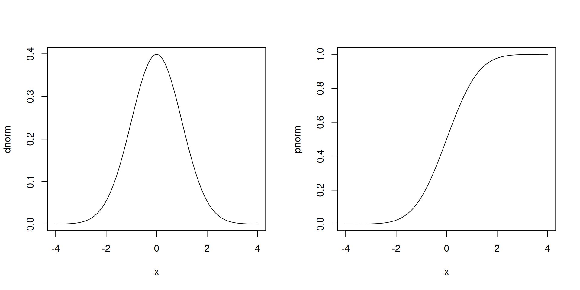
The standard normal distribution has some nice properties:

• Its pdf is symmetric about zero. The curve has a peak at 0.
• One unit to the left and the right of zero: inflection points, PDF curve changes concavity
• The area between -1 to 1 is roughly 68%. The area between -2 to 2 is roughly 95%. The area between -3 to 3 is roughly 99.7%.
• Typically, probabilities from the standard normal are obtained from a table or from software.

par(mfrow=c(1,2)) # only for design purposes
plot(dnorm, from = -4, to = 4)
plot(pnorm, from = -4, to = 4)

What does the red curve buy us?

1. We can now calculate probabilities involving the sample mean by directly using a large-sample approximation.

2. To be more specific, suppose we want to know \(\mathbb{P}\left(\overline{X}_{20} \leq 4.3\right)\) when we have IID random variables \(X_1,\ldots, X_{20}\) from the distribution \(\mathbb{P}\left(X=2\right)=1/10\), \(\mathbb{P}\left(X=3\right)=1/10\), \(\mathbb{P}\left(X=5\right)=8/10\).

3. This is not really impossible to compute, but it is extremely tedious to construct distribution of \(\overline{X}_{20}\).

4. In fact, you can find the requested probability directly by simulation.

a <- replicate(10^4, sample(c(2, 3, 5), 20, prob = c(0.1, 0.1, 0.8), replace = TRUE))
sample.means <- colMeans(a)
mean(sample.means <= 4.3)

[1] 0.222

5. You can also use Chebyshev’s inequality to give an extremely rough check and it works regardless of the value of \(n\).
6. Unfortunately, Chebyshev’s inequality gives an upper bound (which may not be very useful).
7. So having a large-sample approximation might be a good compromise.

Theorem 2 (The Central Limit Theorem (Wasserman (2004) p.77, Theorem 5.8)) Suppose \(X_1, \ldots, X_n\) are IID random variables with mean \(\mathbb{E}(X_i)=\mu\) and \(\mathsf{Var}\left(X_i\right)=\sigma^2\). Then, \[Z_n=\frac{\overline{X}_n-\mathbb{E}\left(\overline{X}_n\right)}{\sqrt{\mathsf{Var}\left(\overline{X}_n\right)}}=\frac{\sqrt{n}\left(\overline{X}_n-\mu\right)}{\sigma}\overset{d}{\to} Z\] where \(Z\sim N(0,1)\). In other words, \[\lim_{n\to\infty}\mathbb{P}\left(Z_n\leq z\right)=\Phi(z).\]

8. How do we use the theorem so that we can avoid simulation?

9. Observe that \[\begin{eqnarray*}\mathbb{P}\left(\overline{X}_{20} \leq 4.3\right) &=& \mathbb{P}\left(Z_{20} \leq \frac{4.3-4.5}{\sqrt{1.05/20}}\right) \\ &=&\mathbb{P}\left(Z_{20}\leq -0.87\right)\end{eqnarray*}\]

10. By the central limit theorem, we can approximate \(\mathbb{P}\left(Z_{20}\leq -0.87\right)\) using \(\mathbb{P}\left(Z\leq -0.87\right)\).

11. We can look the latter probability up from a standard normal table or use R.

pnorm((4.3-4.5)/sqrt(1.05/20))

[1] 0.191

12. Does it match the simulation result well? Not really and an explanation is that \(n\) is not “large enough” for the approximation to kick in.

13. Let us find \(\mathbb{P}\left(\overline{X}_{30} \leq 4.3\right)\) using simulation:

a <- replicate(10^4, sample(c(2, 3, 5), 30, prob = c(0.1, 0.1, 0.8), replace = TRUE))
sample.means <- colMeans(a)
mean(sample.means <= 4.3)

[1] 0.161

14. Now, based on the central limit theorem: \[\mathbb{P}\left(Z_{30}\leq \frac{4.3-4.5}{\sqrt{1.05/30}}\right) \approx \mathbb{P}\left(Z\leq -1.07\right)\]

pnorm((4.3-4.5)/sqrt(1.05/30))

[1] 0.143

15. Let us find \(\mathbb{P}\left(\overline{X}_{40} \leq 4.3\right)\) using simulation:

a <- replicate(10^4, sample(c(2, 3, 5), 40, prob = c(0.1, 0.1, 0.8), replace = TRUE))
sample.means <- colMeans(a)
mean(sample.means <= 4.3)

[1] 0.128

16. Now, based on the central limit theorem: \[\mathbb{P}\left(Z_{40}\leq \frac{4.3-4.5}{\sqrt{1.05/40}}\right) \approx \mathbb{P}\left(Z\leq -1.23\right)\]

pnorm((4.3-4.5)/sqrt(1.05/40))

[1] 0.109

17. Let us find \(\mathbb{P}\left(\overline{X}_{50} \leq 4.3\right)\) using simulation:

a <- replicate(10^4, sample(c(2, 3, 5), 50, prob = c(0.1, 0.1, 0.8), replace = TRUE))
sample.means <- colMeans(a)
mean(sample.means <= 4.3)

[1] 0.0947

18. Now, based on the central limit theorem: \[\mathbb{P}\left(Z_{50}\leq \frac{4.3-4.5}{\sqrt{1.05/50}}\right) \approx \mathbb{P}\left(Z\leq -1.38\right)\]

pnorm((4.3-4.5)/sqrt(1.05/50))

[1] 0.0838

19. The central limit theorem approximation is getting a bit better.

    • Note that you have to skeptical of people saying \(n\geq 30\) is a large sample size. It depends on the situation.
    • You just have to think about how we use 10000 replications in simulation settings to reinforce your skepticism.

20. Just like Chebyshev’s inequality we do not really need to know fully the common distribution of each of \(X_i\)’s. We only need to know the common mean, common variance, and the sample size.