Lecture 6c

Vignettes, moving forward

Andrew Pua

2024-12-02

Other decision rules in hypothesis testing

1. Some prefer using a “critical value” approach to hypothesis testing.
2. The underlying idea may just be as natural as the \(p\)-value approach you have seen so far.
3. The difference is that any other reader of your test results may have their own \(\alpha\) and reporting your \(p\)-value gives other readers some flexibility.

4. Suppose you want to test the null that \(\mu=5\) against \(\mu>5\) for whatever legitimate reason. The idea is to design a decision rule like “Reject the null whenever \(\overline{X}_n\) exceeds a threshold” in order to achieve control of the probability of a Type I error.

5. The question is how to determine the threshold. The central limit theorem can be useful here once more.

Central limit theorem after a plug-in

1. Recall that \(S_n\) is the sample standard deviation. It is not an unbiased estimator of \(\sigma\), but it is a consistent estimator of \(\sigma\).

Theorem 1 (Wasserman (2004) p.78, Theorem 5.10)) Suppose \(X_1, \ldots, X_n\) are IID random variables with mean \(\mathbb{E}(X_i)=\mu\) and \(\mathsf{Var}\left(X_i\right)=\sigma^2\). Then, \[Z_n=\frac{\sqrt{n}\left(\overline{X}_n-\mu\right)}{S_n}\overset{d}{\to} N(0,1)\]

2. But as demonstrated before, we really need a large sample for the result to really “kick in”.
3. Of course, what large means depends on the distribution of the data.
4. You will learn other central limit theorems for other estimators, perhaps not as explicitly.

Moving on to more realistic cases

1. Moving beyond Theorem 1 of Lecture 5d, the weak law of large numbers, and the central limit theorem would be the next steps.

2. So far, we focused on a setting where \(X_1, \ldots, X_n\) are IID random variables with \(\mu=\mathbb{E}\left(X_i\right)\), and \(\sigma^2=\mathsf{Var}\left(X_i\right)\).

3. You can extend to random vectors and then study vector of parameters or even parameters that quantify relationships between elements of a random vector.

4. You can drop independence, but things get complicated quickly. What happens to \(\mathsf{Var}\left(\overline{X}_n\right)\) for example? Venture into time series analysis if interested.
5. You can drop identical distributions, but this becomes a bit more complicated. Venture into clustering if interested.

Linear regression

1. Next term you will learn a method called linear regression.
2. What does it do? Is it connected to what you have learned in this course?

mandm <- read.csv("mandm.csv")
mean(mandm$total_weight)

[1] 14.6537

sd(mandm$total_weight)

[1] 0.5123799

sd(mandm$total_weight)/sqrt(54)

[1] 0.06972608

summary(lm(total_weight ~ 1, data = mandm))

Call:
lm(formula = total_weight ~ 1, data = mandm)

Residuals:
    Min      1Q  Median      3Q     Max 
-1.3537 -0.4037 -0.0037  0.3463  1.5463 

Coefficients:
            Estimate Std. Error t value Pr(>|t|)    
(Intercept) 14.65370    0.06973   210.2   <2e-16 ***
---
Signif. codes:  0 '***' 0.001 '**' 0.01 '*' 0.05 '.' 0.1 ' ' 1

Residual standard error: 0.5124 on 53 degrees of freedom

confint(lm(total_weight ~ 1, data = mandm))

               2.5 %   97.5 %
(Intercept) 14.51385 14.79356

tapply(mandm$total_weight, mandm$scale, mean)

       1        2        3        4        5        6 
14.83077 14.54286 14.84545 14.40000 14.64545 14.30000 

summary(lm(total_weight ~ factor(scale), data = mandm))

Call:
lm(formula = total_weight ~ factor(scale), data = mandm)

Residuals:
     Min       1Q   Median       3Q      Max 
-1.00000 -0.30000 -0.03811  0.30000  1.35455 

Coefficients:
               Estimate Std. Error t value Pr(>|t|)    
(Intercept)    14.83077    0.13832 107.217   <2e-16 ***
factor(scale)2 -0.28791    0.23381  -1.231   0.2242    
factor(scale)3  0.01469    0.20432   0.072   0.9430    
factor(scale)4 -0.43077    0.23381  -1.842   0.0716 .  
factor(scale)5 -0.18531    0.20432  -0.907   0.3689    
factor(scale)6 -0.53077    0.26245  -2.022   0.0487 *  
---
Signif. codes:  0 '***' 0.001 '**' 0.01 '*' 0.05 '.' 0.1 ' ' 1

Residual standard error: 0.4987 on 48 degrees of freedom
Multiple R-squared:  0.1419,    Adjusted R-squared:  0.05255 
F-statistic: 1.588 on 5 and 48 DF,  p-value: 0.1815

Connection to models?

1. In our course, our focus is on models like \[Y_i=\beta_0+\varepsilon_i,\ \mathbb{E}\left(\varepsilon_i\right)=0,\ \mathsf{Var}\left(\varepsilon_i\right)=\sigma^2\] where \(\beta_0\) has a very special meaning.

2. In ECOMETR, you will be looking into models like \[Y_i=\beta_0+\beta_1 X_i+\varepsilon_i\] with suitable assumptions about \(\varepsilon_i\) or \(\beta_0\), \(\beta_1\), and \(\beta_0+\beta_1X_i\) will also have special meanings.

M&M’s again

1. The record I know is as follows: In January 2006, the website for M&M candies claimed that 20% of plain M&M candies are orange, 16% green, 14% yellow, 13% each red and brown, and 24% are blue.

2. We want to test whether the data we have collected is compatible with the claim above.

3. Let \(\theta=(\theta_{\mathsf{orange}}, \theta_{\mathsf{green}}, \theta_{\mathsf{yellow}}, \theta_{\mathsf{red}}, \theta_{\mathsf{brown}}, \theta_{\mathsf{blue}})\). \(\theta\) is a parameter representing the probability mass function of a random variable representing color.

4. We want to test the null that \(\theta=(0.2, 0.16, 0.14, 0.13, 0.13, 0.24)\) against the alternative that \(\theta\neq(0.2, 0.16, 0.14, 0.13, 0.13, 0.24)\).

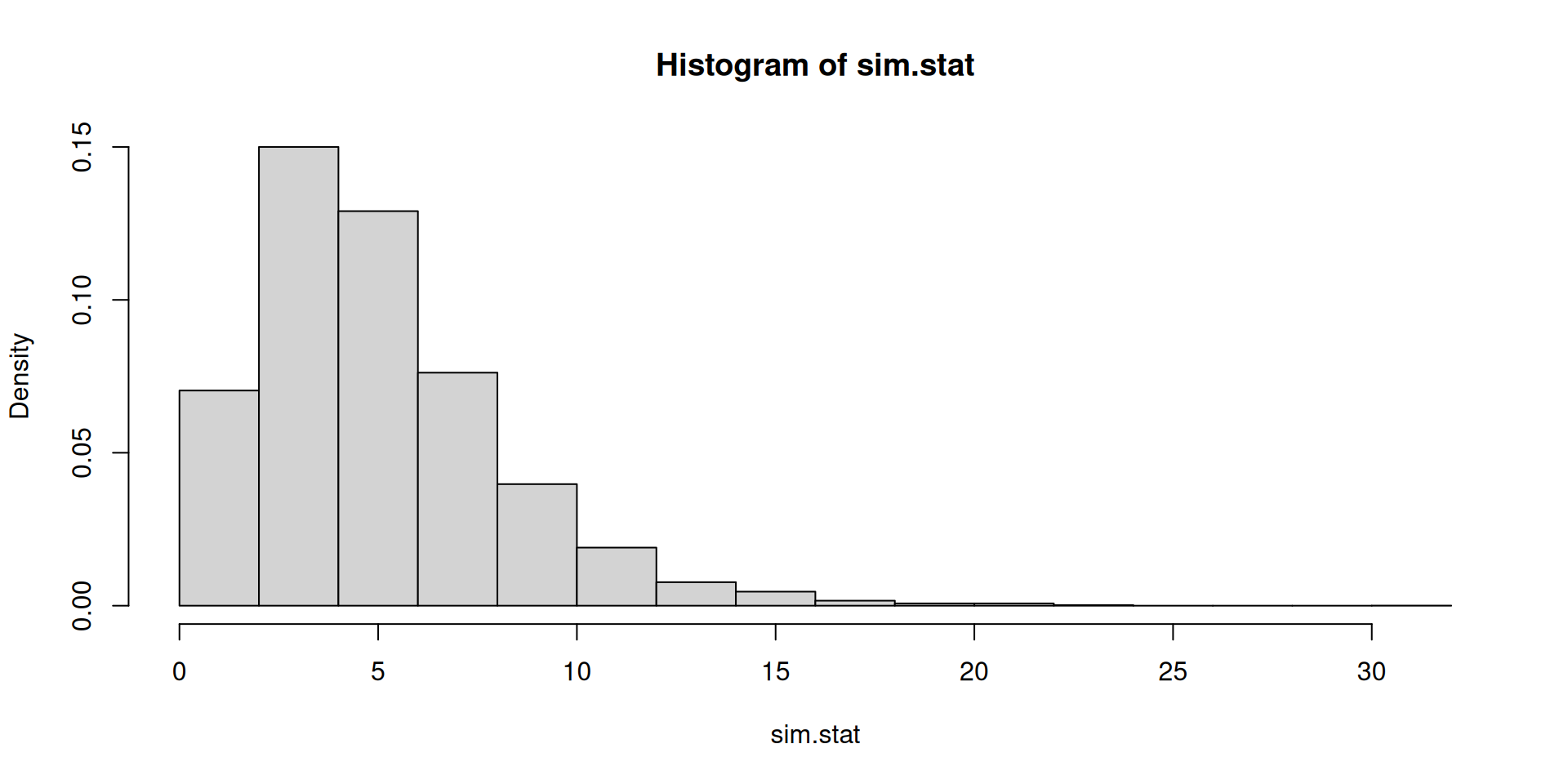
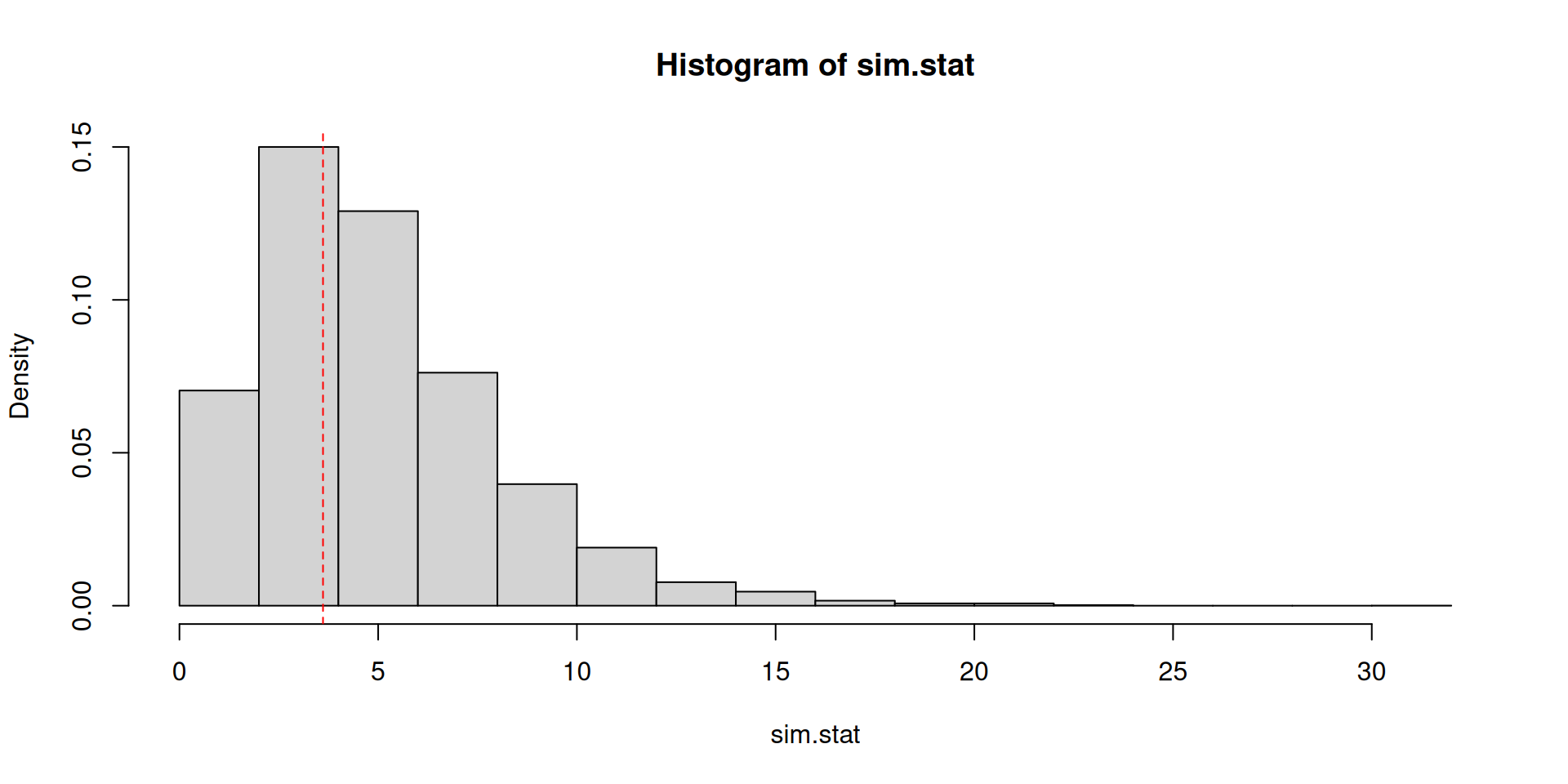
5. It is easy to generate artificial data under the null.

   • But what do you do next?
   • If we are calculating a \(p\)-value, what test statistic should we simulate?

6. To develop a test, the idea is to think about the following test statistic: \[\sum_{\mathsf{all}\ \mathsf{categories}} \frac{\left(\mathsf{observed}\ \mathsf{counts}-\mathsf{expected}\ \mathsf{counts}\right)^2}{\mathsf{expected}\ \mathsf{counts}}\]

7. This is called a Pearson \(\chi^2\) statistic (refer to Wasserman Section 10.3).

observed.counts <- mandm[1, c("n_orange", "n_green", "n_yellow", "n_red", "n_brown", "n_blue")]
observed.counts

  n_orange n_green n_yellow n_red n_brown n_blue
1        2       3        2     3       4      2

observed.counts <- mandm[1, c("n_orange", "n_green", "n_yellow", "n_red", "n_brown", "n_blue")]
observed.counts

  n_orange n_green n_yellow n_red n_brown n_blue
1        2       3        2     3       4      2

expected.counts <- 16*c(0.2, 0.16, 0.14, 0.13, 0.13, 0.24)
expected.counts

[1] 3.20 2.56 2.24 2.08 2.08 3.84

test <- sum((observed.counts-expected.counts)^2/expected.counts)
test

[1] 3.612237

a <- replicate(10^4, sample(c(1, 2, 3, 4, 5, 6), 16, prob = c(0.2, 0.16, 0.14, 0.13, 0.13, 0.24), replace = TRUE))
calc.stat <- function(data)
{
  obs_n <- 16
  obs_orange <- sum(data == 1)
  obs_green <- sum(data == 2)
  obs_yellow <- sum(data == 3)
  obs_red <- sum(data == 4)
  obs_brown <- sum(data == 5)
  obs_blue <- sum(data == 6)
  observed.counts <- c(obs_orange, obs_green, obs_yellow, obs_red, obs_brown, obs_blue)
  expected.counts <- obs_n*c(0.2, 0.16, 0.14, 0.13, 0.13, 0.24)
  test <- sum((observed.counts - expected.counts)^2/expected.counts)
  return(test)
}
sim.stat <- apply(a, 2, calc.stat)

hist(sim.stat, freq = FALSE)

mean(sim.stat >= test)

[1] 0.6197

hist(sim.stat, freq = FALSE)
abline(v = test, col = "red", lty = 2)

Distributions related to the standard normal

1. You might encounter other random variables with special distributions.
2. If \(Z \sim N(0,1)\), then \(Z^2\) has a chi-squared (\(\chi^2\)) distribution with one degree of freedom (df). Usually written as \(Z^2\sim\chi^2_1\).
3. If \(Z_1,\ldots, Z_k\) are IID standard normal random variables, then \(Z_1^2+\cdots+Z_k^2 \sim \chi^2_k\).

4. If \(Z\sim N(0,1)\), \(W\sim\chi^2_k\), and \(Z\) is independent of \(W\), then \(\dfrac{Z}{W/k}\) has a \(t\)-distribution with \(k\) degrees of freedom.
5. If \(W_1 \sim \chi^2_{k_1}\), \(W_2 \sim \chi^2_{k_2}\), and \(W_1\) and \(W_2\) are independent, then \(\dfrac{W_1/k_1}{W_2/k_2}\) has an F-distribution with \(k_1\) numerator degrees of freedom and \(k_2\) denominator degrees of freedom.

6. As \(k\to \infty\), probabilities based on the \(t\)-distribution can be approximated by probabilities based on \(N(0,1)\).
7. As \(k_2\to \infty\), probabilities based on the \(k_1 \times\) \(F\)-distribution can be approximated by probabilities based on \(\chi^2_{k_1}\).

Estimation methods

1. In practice, there are broadly three estimation approaches used in economics:

   • The method of least squares (subject of ECOMETR, here as lm() command)
   • The method of moments (you actually have been using this in the background)
   • The method of maximum likelihood (joint pmf’s and pdf’s are a starting point)

2. You actually are using method of moments without even realizing it.

   • When we use the sample mean to estimate a population mean
   • A suitable law of large numbers justifies the use of the method of moments
   • In our case: we have a so-called moment function \(g(X, \mu) = X-\mu\) such that this function is subject to a restriction: \[\mathbb{E}\left(g(X_i, \mu)\right)=\mathbb{E}\left(X_i-\mu\right)=0\]

3. The method was already around during the 1880s.
4. It is so useful in economics that some economic models generate moment restrictions.
5. Around the late 70s and early 80s, the generalized method of moments was invented as part of economics!
6. To learn more, I have a recent presentation about the method of moments here, if you are interested.

Bootstrap

1. Try using the computer to obtain a standard error even if the theory-based standard error may be hard to obtain

   • Recall that the standard error of the sample mean is the standard deviation of the sampling distribution of the sample mean.
   • Recall that we derived these standard errors using theory.
   • Finally, recall that we have been using Monte Carlo simulations to get a sense of whether the formulas obtained by direct analytical calculation are accurate.

Sample size \(n=50\), number of resamples \(B=200\)

data <- sample(c(2, 3, 5), 50, prob = c(0.1, 0.1, 0.8), replace = TRUE)
data

 [1] 5 5 3 5 3 5 5 5 5 5 2 2 5 3 5 3 3 5 2 5 2 5 5 5 5 2 5 3 5 5 2 5 5 5 5 5 5 5
[39] 5 5 5 2 5 5 2 5 5 2 5 5

mean(data)

[1] 4.22

resamples <- replicate(200, sample(data, replace = TRUE))
collect.means <- apply(resamples, 2, mean)
sd(collect.means)

[1] 0.1764338

# Does it match the theoretical standard error?
sqrt(1.05)/sqrt(50)

[1] 0.1449138

Sample size \(n=100\), number of resamples \(B=200\)

data <- sample(c(2, 3, 5), 100, prob = c(0.1, 0.1, 0.8), replace = TRUE)
data

  [1] 5 5 3 2 5 5 5 5 5 5 5 5 5 5 2 5 5 5 5 5 5 5 3 3 5 3 3 5 5 5 5 5 3 5 5 5 5
 [38] 5 3 5 5 5 5 5 5 5 5 5 5 5 5 5 5 5 3 5 5 5 2 5 5 5 5 3 5 5 3 5 5 5 5 5 5 3
 [75] 5 3 5 5 3 5 5 5 3 3 5 5 5 2 5 5 5 5 5 5 5 2 5 5 5 5

mean(data)

[1] 4.55

resamples <- replicate(200, sample(data, replace = TRUE))
collect.means <- apply(resamples, 2, mean)
sd(collect.means)

[1] 0.09962134

# Does it match the theoretical standard error?
sqrt(1.05)/sqrt(100)

[1] 0.1024695

2. As an exercise, try repeating the code above on your own computer. What changed? What did not change?

3. What we have done is called the nonparametric bootstrap.

4. Notice that if we did not know how to derive the theoretical standard error of \(\sigma/\sqrt{n}\), we would not know what standard error to report. We also may not be able to compute confidence intervals or test hypotheses. Therefore, having a tool like the bootstrap actually helps in practice.

5. Natural questions to ask include:

   • What if I know the distribution that generated the data but do not know its parameters?
   • Is there a bootstrap version of obtaining confidence intervals and testing hypotheses directly?
   • You may also wonder why did we not look at mean(collect.means). Is there something to learn from mean of the estimates obtained from the resampled data?

6. Other questions to ask and explore

   • What if you have other estimators in mind, say functions of the sample mean?
   • Does it work all the time? When will it not work?
   • Did we actually create new datasets as a result of resampling?

7. To learn more and to see different versions of the bootstrap, feel free to explore using my notes here.

Wrap up

1. People are always excited with handling data.

   • But they don’t think about what to do with the data first before touching it.
   • There is room for exploration but exploration can sometimes color our judgments and the way we approach questions.
   • Learn the distinction between knowing how to execute commands and how to even decide which commands to execute.

2. The course placed emphasis on

   • using simulation for understanding the performance of statistical procedures
   • using simulation for testing hypotheses
   • understanding both conceptually and mathematically how probability theory and random variables play roles in statistics

3. The course reduced emphasis on

   • normal distributions and bell-shapedness, but this was useful when thinking about statistical procedures based on large samples
   • continuous distributions, but this will be very useful in finance settings
   • going through a laundry list of tests and procedures

4. If you want more realistic datasets, I would recommend the following resource, but you may have to do some modifications to be able to make things work.

   • For example, the code has to be modified to point to the correct location of the data.
   • You may want to start using a local version of R rather than Google Colab.
   • You may have to install packages and learn more about your computer system in the process.